Flow Matching in PyTorch: Train a Model to Follow a Straight Line
Where you are: Post 8 of 14 in PyTorch Tutorial 2026 · about 13 min read
What you’ll build: tinydit/flow.py: the flow-matching loss and the Euler sampler, tested on a 2D “two moons” toy you can watch. The next post uses the exact same two functions to train TinyDiT on images.
You’ll need: Post 2 (broadcasting), Post 3 (torch.no_grad), Post 5 (Trainer) and Post 7 (TinyDiT’s skeleton).
In this post:
- Introduction
- Step 1/6: The Big Idea: A Straight Line from Data to Noise
- Step 2/6: Flow Matching in PyTorch: The Training Loss
- Step 3/6: The Sampler: Euler Steps from Noise to Data
- Step 4/6: A 2D Toy You Can See
- Step 5/6: Why Doesn't the Loss Go to Zero?
- Step 6/6: Why Flow Matching Instead of DDPM?
- Recap
Series: PyTorch Tutorial 2026 (14 posts)
- Post 1: PyTorch Tutorial 2026: From Tensors to Tiny Diffusion
- Post 2: PyTorch Tensors Explained: Shapes, Broadcasting, and Images as Arrays
- Post 3: PyTorch Autograd: How backward() Builds Gradients
- Post 4: PyTorch DataLoader Explained: Datasets, Batches, and Image Folders
- Post 5: PyTorch nn.Module and the Training Loop: Layers, Loss, and Checkpoints
- Post 6: Attention and the Transformer Block in PyTorch
- Post 7: Patch Embeddings in PyTorch: How a Transformer Reads an Image
- Post 8: Flow Matching in PyTorch: Train a Model to Follow a Straight Line (you are here)
- Post 9: Build a Tiny Diffusion Transformer in PyTorch (DiT from Scratch)
- Post 10: torch.compile, Mixed Precision, and SDPA: Speed Up TinyDiT
- Post 11: RMSNorm, QK-Norm, SwiGLU, and 2D RoPE in a Tiny DiT
- Post 12: adaLN-Zero and Classifier-Free Guidance in PyTorch
- Post 13: MMDiT Joint Attention in PyTorch: Two Streams, One Generator
- Post 14: Train and Sample Like 2026: Logit-Normal Steps, EMA, and Few-Step Flow
Introduction
Up to now our models could only clean a picture. A generator has to do something harder: start from pure random noise and end up with a picture. Today we learn the idea that makes that possible, and it is surprisingly small.
In this flow matching PyTorch tutorial we draw a straight line from a data point to a noise point, train a network to predict the direction along that line, and then walk backward from noise to data in a few small steps. We write the loss and the sampler once, in tinydit/flow.py, test them on a 2D toy you can watch, and in the next post the exact same two functions train TinyDiT on real images.
In Patch Embeddings in PyTorch: How a Transformer Reads an Image we finished TinyDiT’s skeleton: image in, tokens through transformer blocks, image out. What it was missing was a job that turns it into a generator. Flow matching is that job.
Step 1/6: The Big Idea: A Straight Line from Data to Noise
In this step: We draw a straight line between a data point and a noise point and find the velocity along it.
Pick one training image, call it x_0. Pick one random noise image of the same shape, call it x_1. Now draw the straight line between them. Every point on that line is a mix of the two:
\begin{gathered} \underbrace{x_t}_{\text{point at time } t} = \underbrace{(1 - t)}_{\text{how much data}}\, \underbrace{x_0}_{\text{data}} + \underbrace{t}_{\text{how much noise}}\, \underbrace{x_1}_{\text{noise}} \\ x_1 \sim \mathcal{N}(0, I),\;\; t \in [0, 1] \end{gathered}At t = 0 we’re at the clean image, at t = 1 we’re at pure noise, and at t = 0.5 it’s half and half. If you move along the line, how fast and in which direction are you going? Take the derivative with respect to t:
\begin{gathered} \underbrace{v}_{\text{velocity}} = \frac{d x_t}{d t} = \underbrace{x_1 - x_0}_{\text{noise minus data}} \\ \text{(the same at every } t \text{: a straight line has one direction)} \end{gathered}That’s the velocity. It doesn’t depend on t at all, because the path is straight. Let’s check it with two numbers:
import torch
from tinydit.flow import interpolate

x0 = torch.tensor([[1.0, 0.5]])     # one "data" point
x1 = torch.tensor([[-0.3, 1.2]])    # one "noise" point
v = x1 - x0                          # the velocity: the same at every t
print("velocity v = x1 - x0:", v.tolist())

for t in [0.0, 0.25, 0.5, 0.75, 1.0]:
    xt = interpolate(x0, x1, torch.tensor([t]))
    print(f"t={t:.2f}  x_t={[round(a, 3) for a in xt[0].tolist()]}")

# Walking backward: start at the noise (t=1) and take 4 steps of dt = -0.25 along v
x = x1.clone()
for _ in range(4):
    x = x + (-0.25) * v
print("after 4 Euler steps from noise:", [round(a, 3) for a in x[0].tolist()], "(back at x0)")

# The same function works on image batches: t has shape (N,), images (N, 3, 32, 32)
imgs, noise, t = torch.randn(4, 3, 32, 32), torch.randn(4, 3, 32, 32), torch.tensor([0.0, 0.3, 0.7, 1.0])
xt = interpolate(imgs, noise, t)
print("image batch x_t:", tuple(xt.shape),
"| t=0 equals data:", torch.equal(xt[0], imgs[0]), "| t=1 equals noise:", torch.equal(xt[3], noise[3]))velocity v = x1 - x0: [[-1.2999999523162842, 0.7000000476837158]]
t=0.00 x_t=[1.0, 0.5]
t=0.25 x_t=[0.675, 0.675]
t=0.50 x_t=[0.35, 0.85]
t=0.75 x_t=[0.025, 1.025]
t=1.00 x_t=[-0.3, 1.2]
after 4 Euler steps from noise: [1.0, 0.5] (back at x0)
image batch x_t: (4, 3, 32, 32) | t=0 equals data: True | t=1 equals noise: TrueThe point moves the same amount every quarter step, and walking backward along v from the noise lands exactly on the data point. This is the whole trick: if someone gave us v at every point, we could start from noise and walk back to data.
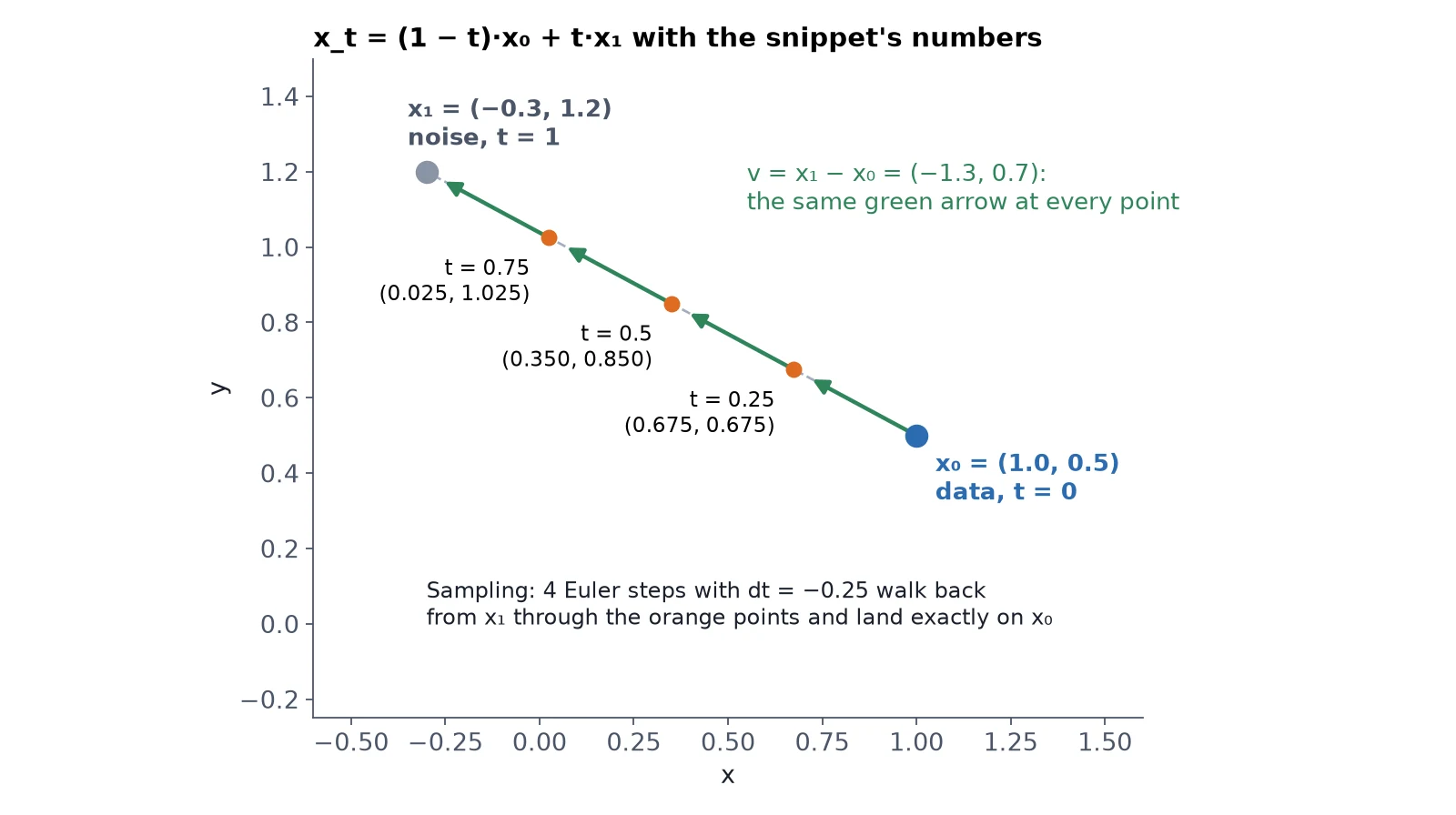
What you just built: The straight-line path x_t = (1 – t)x_0 + t x_1 and its constant velocity v = x_1 – x_0, checked with numbers.
Step 2/6: Flow Matching in PyTorch: The Training Loss
In this step: We turn the straight line into a training objective: the network predicts the velocity, and MSE compares it with x_1 – x_0.
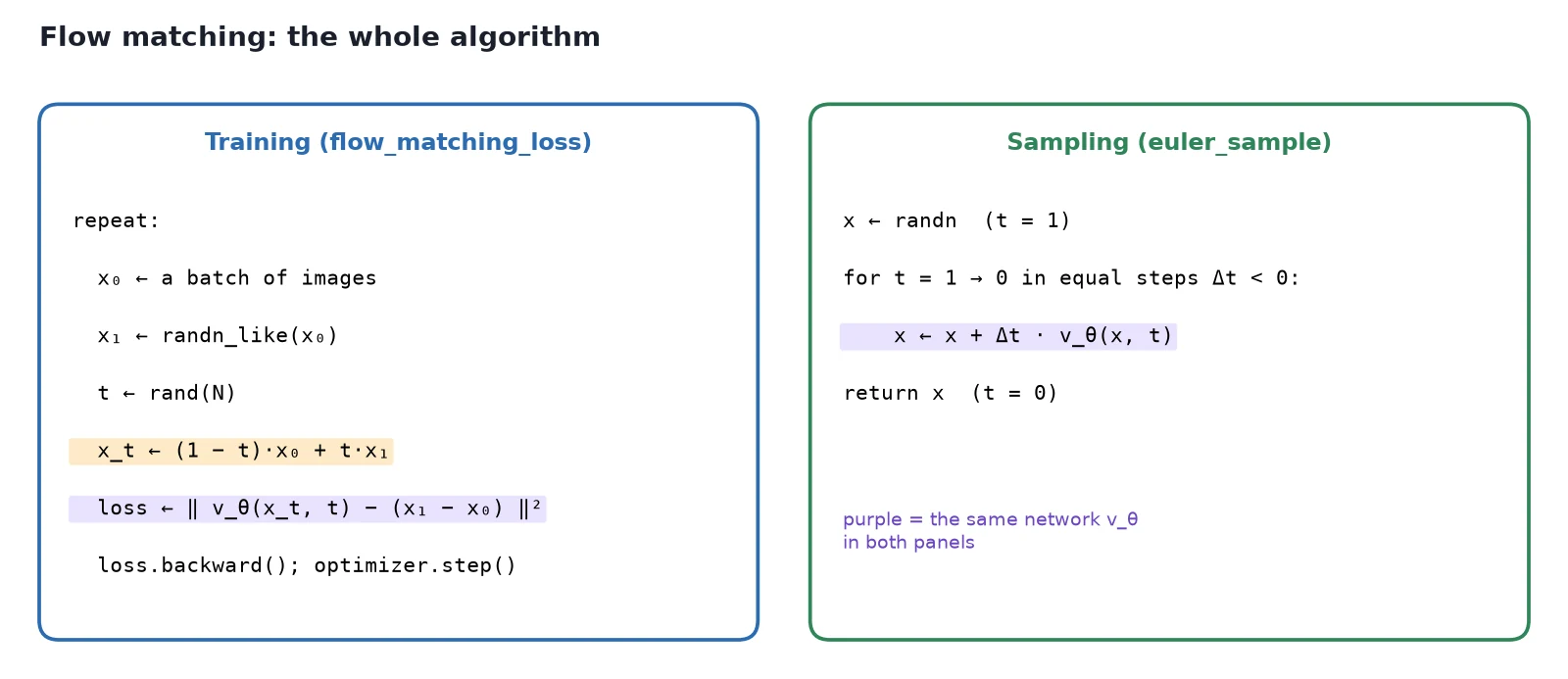
Of course, at generation time nobody tells us which x_0 we’re heading to. That’s what the network learns. We show it a point x_t and the time t, and ask it to predict the velocity v_\theta(x_t, t). The loss is plain mean squared error against the true velocity:
\begin{gathered} \mathcal{L}(\theta) = \mathbb{E} \Big[ \big\| \underbrace{v_\theta(x_t, t)}_{\text{network's guess}} - \underbrace{(x_1 - x_0)}_{\text{true velocity}} \big\|^2 \Big] \\ x_0 \sim \text{data},\;\; x_1 \sim \mathcal{N}(0, I),\;\; t \sim U[0, 1] \end{gathered}In words, each training step does five things:
- Take a batch of data x_0.
- Draw a noise batch x_1 of the same shape.
- Draw a random time t for each sample, uniformly between 0 and 1.
- Mix them: x_t = (1 – t)x_0 + t x_1.
- Ask the model for the velocity at (x_t, t) and compare it with x_1 – x_0 using MSE.
This objective was introduced as flow matching by Lipman and colleagues (Flow Matching for Generative Modeling, ICLR 2023) and, from a different angle, as rectified flow by Liu, Gong and Liu (Flow Straight and Fast, ICLR 2023). Stable Diffusion 3 (Esser et al., 2024) and FLUX train with it, using this very same straight-line convention: t = 0 is data, t = 1 is noise.
The code, piece by piece
Here’s our implementation, tinydit/flow.py. It opens with the convention and two helpers: expand_t for broadcasting and interpolate for the straight line:
"""Flow matching: the training loss and the Euler sampler (post 8).

Convention (same as SD3 / rectified flow):
  x_0 = data, x_1 = Gaussian noise, t in [0, 1]
  x_t = (1 - t) * x_0 + t * x_1            (a straight line)
  v   = d x_t / d t = x_1 - x_0            (constant along the line)
A model predicts v from (x_t, t). Sampling integrates dx/dt = v from t = 1 (noise) to t = 0 (data).

Model call convention: model(x_t, t) or, when conditional=True, model(x_t, t, y).
"""
import torch
import torch.nn.functional as F
from torch import nn


def expand_t(t: torch.Tensor, x: torch.Tensor) -> torch.Tensor:
    """(N,) -> (N, 1, 1, ...) so it broadcasts against x."""
    return t.reshape(-1, *([1] * (x.dim() - 1)))


def interpolate(x0: torch.Tensor, x1: torch.Tensor, t: torch.Tensor) -> torch.Tensor:
    """Point on the straight line from data x0 (t=0) to noise x1 (t=1)."""
    t = expand_t(t, x0)
return (1 - t) * x0 + t * x1expand_t is a small broadcasting helper. t has shape (N,), one time per sample, but images have shape (N, 3, 32, 32). Reshaping t to (N, 1, 1, 1) lets broadcasting (post 2) mix every pixel of sample i with the same t_i, which is why the same interpolate worked on both 2D points and image batches in step 1.
sample_t draws the training times. The default is uniform; the logit-normal option is for post 14:
def sample_t(n: int, device=None, dist: str = "uniform", mean: float = 0.0, std: float = 1.0,
             generator: torch.Generator | None = None) -> torch.Tensor:
    """Training times. 'uniform': U(0, 1). 'logit_normal': sigmoid(N(mean, std)) as in SD3 (post 14)."""
    if dist == "uniform":
        return torch.rand(n, device=device, generator=generator)
    if dist == "logit_normal":
        return torch.sigmoid(mean + std * torch.randn(n, device=device, generator=generator))
raise ValueError(f"unknown t distribution {dist!r}")FlowMatchingLoss is the five steps above. Its extra options switch on class labels in post 12; with the defaults they do nothing:
class FlowMatchingLoss:
    """loss_fn(model, batch) for the Trainer. batch = (x0, y).

    conditional: pass labels y to the model (post 12+).
    drop_prob:   replace y by `null_class` with this probability (classifier-free guidance, post 12).
    """

    def __init__(self, t_dist: str = "uniform", ln_mean: float = 0.0, ln_std: float = 1.0,
                 conditional: bool = False, drop_prob: float = 0.0, null_class: int | None = None):
        self.t_dist, self.ln_mean, self.ln_std = t_dist, ln_mean, ln_std
        self.conditional, self.drop_prob, self.null_class = conditional, drop_prob, null_class

    def __call__(self, model: nn.Module, batch) -> torch.Tensor:
        x0, y = batch
        x1 = torch.randn_like(x0)                                   # noise
        t = sample_t(x0.shape[0], x0.device, self.t_dist, self.ln_mean, self.ln_std)
        xt = interpolate(x0, x1, t)
        target = x1 - x0                                            # velocity
        if self.conditional:
            if self.drop_prob > 0:
                drop = torch.rand(y.shape[0], device=y.device) < self.drop_prob
                y = torch.where(drop, torch.full_like(y, self.null_class), y)
            pred = model(xt, t, y)
        else:
            pred = model(xt, t)
        return F.mse_loss(pred, target)


flow_matching_loss = FlowMatchingLoss() # the plain post-8 loss: uniform t, unconditionalNotice that flow_matching_loss(model, batch) has the same signature as the losses from post 5, so it plugs straight into our Trainer. The batch is (x0, y), the same thing our DataLoaders yield. The labels are ignored for now.
The flow-matching objective: what, why, how
What it is: a way of teaching a network the direction from noise to data at every point and time.
Why it works: a straight line between a data point and a noise point has one fixed velocity, x_1 – x_0, which is easy to compute and easy to regress. When many lines cross, MSE makes the network learn their average, and that averaged field still moves the whole noise distribution onto the data distribution (Lipman et al., 2023; Liu et al., 2023).
How it works: x1 = torch.randn_like(x0), t = torch.rand(N), xt = (1 - t) * x0 + t * x1, then F.mse_loss(model(xt, t), x1 - x0). In our repo: FlowMatchingLoss and flow_matching_loss in tinydit/flow.py.
What you just built: FlowMatchingLoss and flow_matching_loss in tinydit/flow.py, ready to plug into the Trainer.
Step 3/6: The Sampler: Euler Steps from Noise to Data
In this step: We write the sampler that turns noise into data by following the model’s velocity backward in small Euler steps.
Once the model knows the velocity, generating is just following it backward. We start at pure noise (t = 1) and take small steps toward t = 0. The simplest way to follow a velocity is Euler’s method: look at the arrow where you stand, take a small step along it, and repeat.
\underbrace{x_{t - \Delta t}}_{\text{next point}} = \underbrace{x_t}_{\text{where we are}} - \underbrace{\Delta t}_{\text{step size, e.g. } 1/20}\; \underbrace{v_\theta(x_t, t)}_{\text{model's arrow}}That’s euler_sample. The cfg_scale branch is for classifier-free guidance in post 12; for now y is None:
@torch.no_grad()
def euler_sample(model: nn.Module, noise: torch.Tensor, steps: int = 20, y: torch.Tensor | None = None,
                 cfg_scale: float = 1.0, null_class: int | None = None,
                 return_path: bool = False):
    """Integrate from t=1 (noise) to t=0 (data) with `steps` equal Euler steps.

    y=None: unconditional. With y and cfg_scale != 1: classifier-free guidance (post 12),
    v = v_uncond + cfg_scale * (v_cond - v_uncond).
    """
    was_training = model.training
    model.eval()
    x = noise
    ts = torch.linspace(1.0, 0.0, steps + 1, device=noise.device)
    path = [x]
    for i in range(steps):
        t = ts[i].expand(x.shape[0])
        if y is None:
            v = model(x, t)
        elif cfg_scale == 1.0:
            v = model(x, t, y)
        else:
            v_c = model(x, t, y)
            v_u = model(x, t, torch.full_like(y, null_class))
            v = v_u + cfg_scale * (v_c - v_u)
        x = x + (ts[i + 1] - ts[i]) * v          # dt is negative: we walk back toward data
        if return_path:
            path.append(x)
    model.train(was_training)
return (x, path) if return_path else xtorch.linspace(1, 0, steps + 1) makes the time grid, and each step does x = x + (t_next - t) * v. Because t_next - t is negative, we move against the arrow, from noise toward data.
Note: The function is decorated with @torch.no_grad() because sampling never needs gradients (post 3), and it switches the model to eval() while it runs.
The Euler sampler: what, why, how
What it is: the procedure that turns noise into data with a trained velocity model.
Why it works: the model gives an arrow at every point. Taking many short steps along the arrows traces the path, and shorter steps follow curves more closely. That’s why 20 steps beat 5, and 1 step fails (step 4).
How it works: start with x = torch.randn(...), walk the time grid torch.linspace(1, 0, steps + 1), and update x = x + (t_next - t) * model(x, t) under torch.no_grad(). In our repo: euler_sample in tinydit/flow.py.
What you just built: euler_sample, which walks from t = 1 (noise) to t = 0 (data) in equal Euler steps.
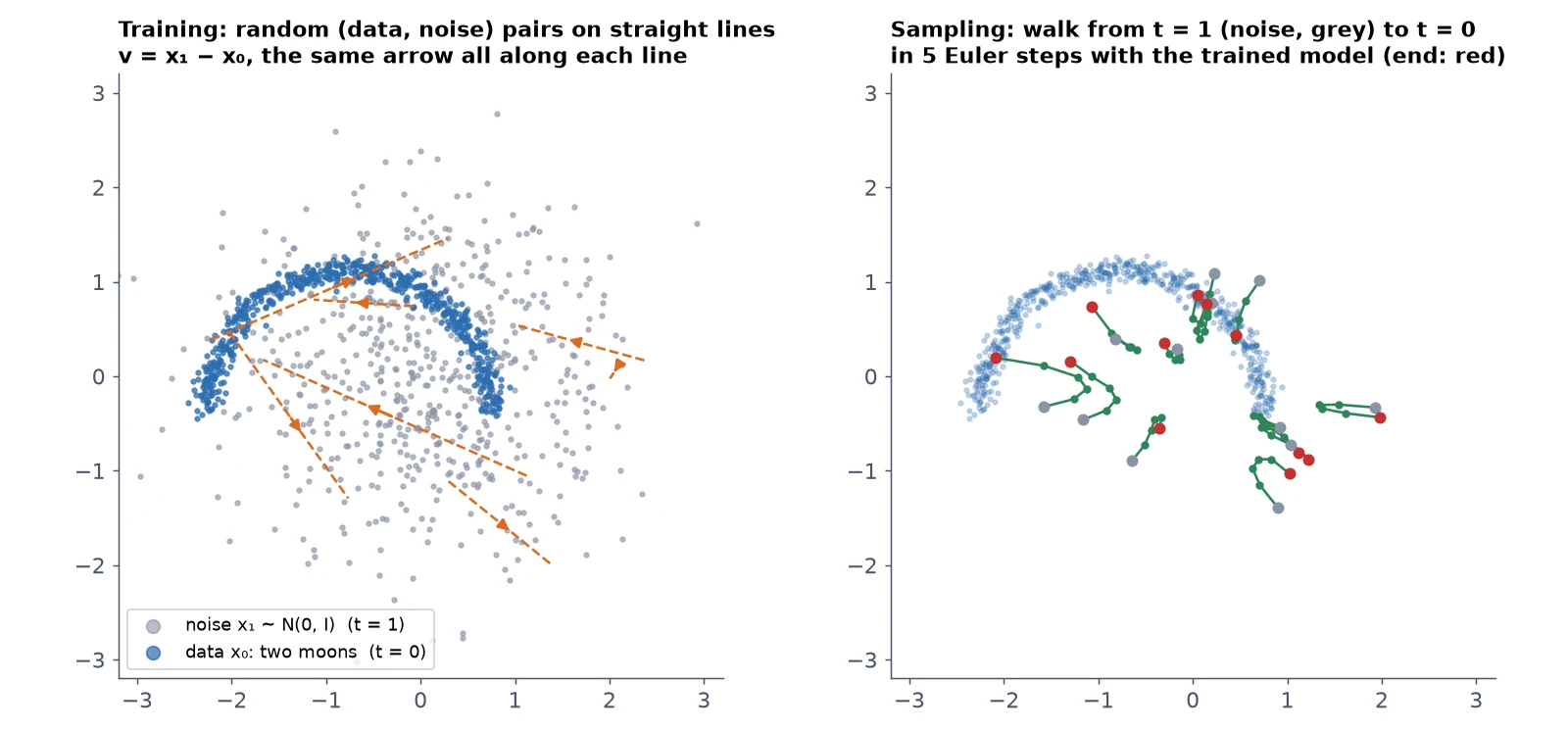
Step 4/6: A 2D Toy You Can See
In this step: We train the real loss and sampler on 2D “two moons” points, where we can see every sample, and score them.
Images have 3,072 numbers each, which is hard to picture. So let’s first train on points in 2D, where we can see everything. Our data is the classic “two moons” shape, made by make_moons in examples/toy2d.py:
"""Flow matching on a 2D toy (post 8): two moons, a small MLP, the real tinydit.flow loss and sampler."""
import math

import torch
from torch import nn


def make_moons(n: int, noise: float = 0.05, generator: torch.Generator | None = None) -> torch.Tensor:
    """n points on two interleaving half circles, shape (n, 2), roughly centred on 0."""
    half = n // 2
    a = torch.rand(half, generator=generator) * math.pi
    b = torch.rand(n - half, generator=generator) * math.pi
    upper = torch.stack([torch.cos(a), torch.sin(a)], dim=1)
    lower = torch.stack([1 - torch.cos(b), 0.5 - torch.sin(b)], dim=1)
    pts = torch.cat([upper, lower]) - torch.tensor([0.5, 0.25])
    pts = pts + noise * torch.randn(pts.shape, generator=generator)
return pts * 1.5 # spread it out so it is comparable to N(0, I) noiseThe model is a tiny MLP that gets the point and the time as input:
class VelocityMLP(nn.Module):
    """(x (N, 2), t (N,)) -> predicted velocity (N, 2). Time is simply fed in as a third input."""

    def __init__(self, hidden: int = 128):
        super().__init__()
        self.net = nn.Sequential(
            nn.Linear(3, hidden), nn.SiLU(),
            nn.Linear(hidden, hidden), nn.SiLU(),
            nn.Linear(hidden, hidden), nn.SiLU(),
            nn.Linear(hidden, 2))

    def forward(self, x: torch.Tensor, t: torch.Tensor) -> torch.Tensor:
return self.net(torch.cat([x, t[:, None]], dim=1))The MLP just glues t on as a third input number. That’s fine for a toy; TinyDiT will need a better way to read the time, which is the first thing we build in post 9.
The file ends with a loader that yields (x0, y) batches like our image loaders, and a score: the mean distance to the true moon curves:
def moons_loader(n_batches: int, batch_size: int = 256, seed: int = 0):
    """A list of (points, dummy_labels) batches, the same (x0, y) shape our image loaders yield."""
    g = torch.Generator().manual_seed(seed)
    return [(make_moons(batch_size, generator=g), torch.zeros(batch_size, dtype=torch.long))
            for _ in range(n_batches)]


@torch.no_grad()
def distance_to_moons(samples: torch.Tensor, n_ref: int = 20000) -> float:
    """Mean distance from each sample to the nearest point of a big, noise-free moons set (lower = better)."""
    ref = make_moons(n_ref, noise=0.0, generator=torch.Generator().manual_seed(123))
return torch.cdist(samples, ref).min(dim=1).values.mean().item()Before training, let’s look at one batch and the starting loss:
import torch
from examples.toy2d import VelocityMLP, moons_loader
from tinydit.flow import flow_matching_loss

torch.manual_seed(0)
model = VelocityMLP()
batch = moons_loader(1)[0]
x0, y = batch
print("one batch:", tuple(x0.shape), "points,", tuple(y.shape), "dummy labels")
print("parameters:", sum(p.numel() for p in model.parameters()))
print("loss before training:", round(flow_matching_loss(model, batch).item(), 4))

# A "know-nothing" guess, v = 0, scores the average of (x1 - x0)^2:
x1 = torch.randn_like(x0)
print("loss of always predicting 0:", round(((x1 - x0) ** 2).mean().item(), 4))one batch: (256, 2) points, (256,) dummy labels
parameters: 33794
loss before training: 2.1288
loss of always predicting 0: 1.9886An untrained network is slightly worse than predicting zero for everything. Now we train it with the Trainer from post 5. Nothing about the loop changes; we just pass the new loss:
import time
import torch
from examples.toy2d import VelocityMLP, moons_loader, make_moons, distance_to_moons
from tinydit.flow import flow_matching_loss, euler_sample
from tinydit.trainer import Trainer

torch.manual_seed(0)
model = VelocityMLP()
trainer = Trainer(model, flow_matching_loss, lr=1e-3)
loader = moons_loader(n_batches=500, batch_size=256)          # 128,000 points, reused
t0 = time.time()
trainer.fit(loader, max_steps=4000, log_every=500, ckpt_path="checkpoints/toy_flow.pt")
print(f"trained in {time.time() - t0:.0f}s on CPU")

noise = torch.randn(2000, 2, generator=torch.Generator().manual_seed(7))
print(f"\nmean distance to the moons (lower is better)")
print(f"  pure noise            : {distance_to_moons(noise):.3f}")
print(f"  real data (noise 0.05): {distance_to_moons(make_moons(2000, generator=torch.Generator().manual_seed(8))):.3f}")
for steps in [1, 2, 5, 20, 100]:
    samples = euler_sample(model, noise, steps=steps)
    torch.save(samples, f"toy_samples_{steps}.pt")
print(f" {steps:3d} Euler steps : {distance_to_moons(samples):.3f}")step 500 | loss 1.6194
step 1000 | loss 1.5169
step 1500 | loss 1.4966
step 2000 | loss 1.4723
step 2500 | loss 1.4741
step 3000 | loss 1.4526
step 3500 | loss 1.4449
step 4000 | loss 1.4347
trained in 247s on CPU
mean distance to the moons (lower is better)
pure noise : 0.445
real data (noise 0.05): 0.060
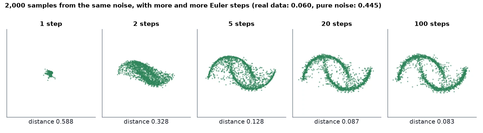
1 Euler steps : 0.588
2 Euler steps : 0.328
5 Euler steps : 0.128
20 Euler steps : 0.087
100 Euler steps : 0.083To judge the samples we measure the average distance from each generated point to the nearest point on the true moon curves. Pure noise scores 0.445. Real data scores 0.060, because it has a little noise of its own.
Our model reaches 0.087 with 20 Euler steps, close to the real data, and barely changes with 100 steps. With 5 steps it’s already decent (0.128).
Watch out: Look at 1 step: 0.588, worse than the noise we started from. Step 5 explains why, because it explains the most surprising thing about flow matching.
The toy VelocityMLP: what, why, how
What it is: a model just for today’s 2D experiment. It is not part of TinyDiT.
Why it works: a few Linear and SiLU layers are plenty to learn a 2D velocity field. Feeding t in as a raw number is the simplest possible time input.
How it works: cat([x, t[:, None]]) → three Linear(128) + SiLU layers → Linear(2).
What you just built: A trained 2D flow-matching model whose 20-step samples land within 0.087 of the true moon curves (real data: 0.060).
Step 5/6: Why Doesn’t the Loss Go to Zero?
In this step: We explain why the loss stays well above zero, why one step fails, and how to check the model on held-out data.
The training loss stopped around 1.43, not near zero. That’s not a bug. It’s built into the problem.
At training time, each line connects one specific data point to one specific noise point. But many different lines pass close to the same spot x_t at the same time t, each with its own direction. The model only sees (x_t, t), so it can’t know which line it’s on.
The best it can do is predict the average direction of all lines through that point. MSE rewards exactly that: the average is the guess with the smallest squared error. The leftover disagreement between lines is error that no model can remove.
Why it works: The beautiful result in the flow-matching papers is that this average is all we need. Following the averaged velocity field from noise still carries the whole cloud of noise onto the whole cloud of data. A single point might not land where “its” training line ended, but the distribution as a whole comes out right.
This also explains the 1-step result. At t = 1 the point is pure noise and says almost nothing about which data point it came from, so the averaged arrow points roughly at the average of the data. One giant step lands every sample in the middle: a blob, not two moons.
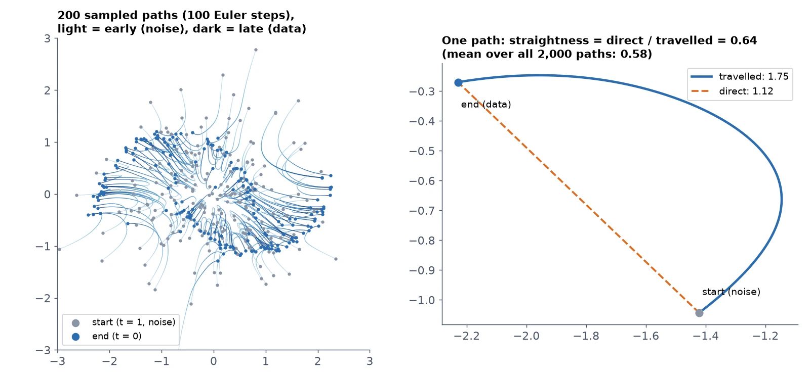
It also means the learned paths are no longer perfectly straight lines. They bend as they get closer to the data and learn more about where they’re going:
import torch
from examples.toy2d import VelocityMLP
from tinydit.flow import euler_sample

model = VelocityMLP()
model.load_state_dict(torch.load("checkpoints/toy_flow.pt", weights_only=True)["model"])

noise = torch.randn(2000, 2, generator=torch.Generator().manual_seed(7))
final, path = euler_sample(model, noise, steps=100, return_path=True)
path = torch.stack(path)                                  # (101 positions, 2000 points, 2)
torch.save(path[:, :200], "toy_paths.pt")

for i in range(3):                                        # follow 3 points from noise to data
    pts = [path[k, i].tolist() for k in (0, 25, 50, 75, 100)]
    print(f"point {i}: " + " -> ".join(f"({a:+.2f},{b:+.2f})" for a, b in pts))

# straightness: straight-line distance / distance actually travelled (1.0 = perfectly straight)
travelled = (path[1:] - path[:-1]).norm(dim=-1).sum(0)
direct = (path[-1] - path[0]).norm(dim=-1)
ratio = direct / travelled
print(f"\nstraightness over 2000 paths: mean {ratio.mean():.3f}, worst {ratio.min():.3f}")point 0: (-0.82,+0.40) -> (-0.68,+0.33) -> (-0.77,+0.35) -> (-1.08,+0.55) -> (-1.51,+0.88)
point 1: (+0.90,-1.39) -> (+0.74,-1.13) -> (+0.78,-0.98) -> (+0.95,-0.94) -> (+1.24,-1.05)
point 2: (-0.17,+0.29) -> (-0.15,+0.22) -> (-0.21,+0.21) -> (-0.30,+0.33) -> (-0.35,+0.62)
straightness over 2000 paths: mean 0.582, worst 0.005A straightness of 1.0 would mean a perfect line. Our paths average 0.58: each one travels noticeably further than the straight distance between its start and end. That’s why we need several steps instead of one.
Note: In post 14 we’ll use reflow, a trick from the rectified-flow paper, to straighten these paths so that a few steps are enough.
How do we check a model on held-out data?
In post 4 we promised a held-out check from this post on. For flow matching, that’s the same loss on data the model never trained on. Because the noise and t are random, the number wobbles a little from run to run, so to compare two models fairly we fix the random seed:
import torch
from examples.toy2d import VelocityMLP, moons_loader
from tinydit.flow import flow_matching_loss
from tinydit.trainer import Trainer

model = VelocityMLP()
trainer = Trainer(model, flow_matching_loss)
trainer.load("checkpoints/toy_flow.pt")
heldout = moons_loader(n_batches=40, batch_size=256, seed=99)    # points the model never saw

for attempt in range(2):        # noise and t are random, so the number wobbles a little
    print(f"held-out velocity MSE, attempt {attempt + 1}: {trainer.evaluate(heldout):.4f}")

torch.manual_seed(0)            # fix the randomness to compare two models fairly
a = trainer.evaluate(heldout)
torch.manual_seed(0)
b = trainer.evaluate(heldout)
print(f"with a fixed seed: {a:.4f} and {b:.4f}")
fresh = Trainer(VelocityMLP(), flow_matching_loss)
torch.manual_seed(0)
print(f"untrained model, same seed: {fresh.evaluate(heldout):.4f}")held-out velocity MSE, attempt 1: 1.4373
held-out velocity MSE, attempt 2: 1.4242
with a fixed seed: 1.4419 and 1.4419
untrained model, same seed: 2.1667The held-out loss (1.44) matches the training loss, so the model didn’t just memorise its batches. In post 9 we’ll use an image version of this with fixed noise and times, called velocity MSE, as one of our main scores.
What you just built: An explanation of the loss floor, the 1-step blob and the bent paths (straightness 0.58), plus a seeded held-out check (1.44).
Step 6/6: Why Flow Matching Instead of DDPM?
In this step: We compare flow matching with the older DDPM recipe and see why TinyDiT, SD3 and FLUX use flow matching.
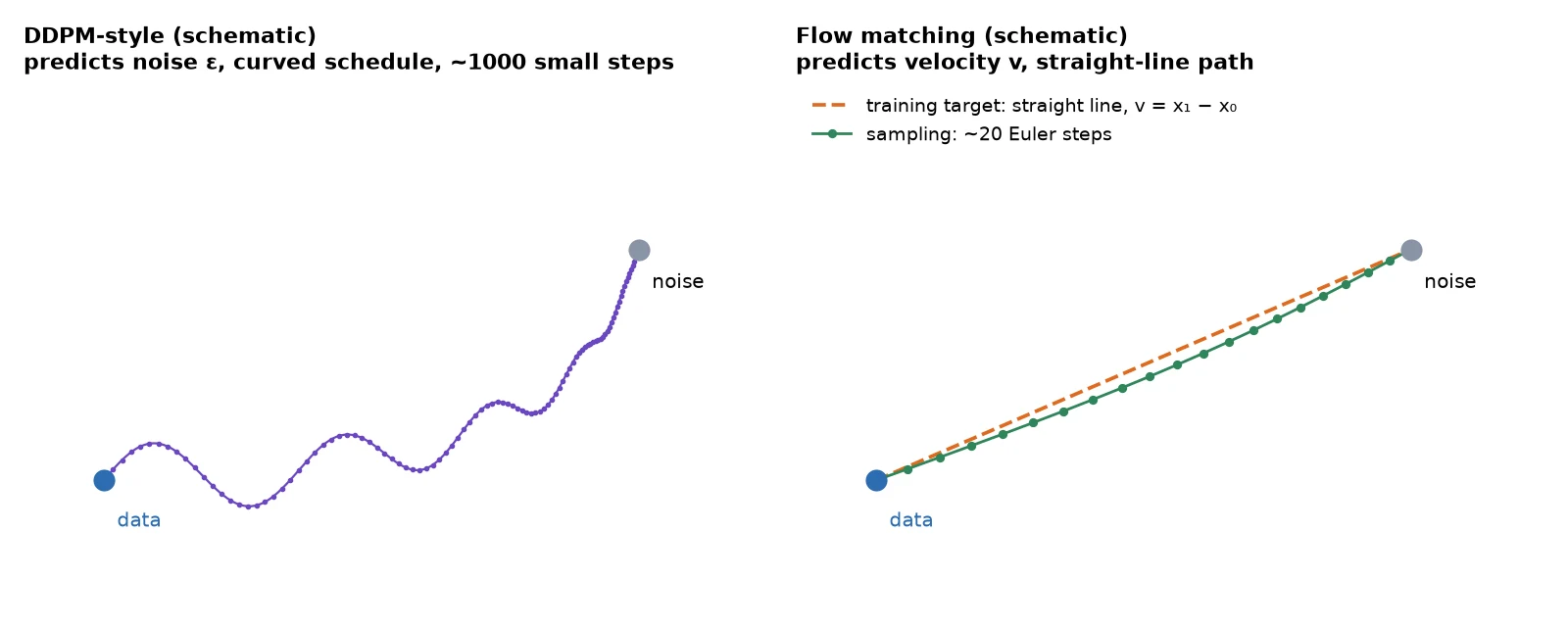
If you’ve read older diffusion tutorials, you’ve seen DDPM (Ho et al., 2020): the model predicts the noise that was added, the noise is added on a curved schedule, and sampling takes hundreds of small steps. It worked, and it powered the first wave of image generators. We’re not going to implement it.
Flow matching keeps the good parts and drops the fiddly ones: one straight path, one MSE loss, no noise schedule to derive, and a sampler that is a plain ODE solver.
Why it works: Ma and colleagues (SiT, ECCV 2024) took the DiT model and only changed the objective to this kind of interpolant, and it improved image quality at the same compute. SD3 and FLUX train this way, which is why TinyDiT does too.
What you just built: A clear reason for the choice of objective: one straight path, one MSE loss, no noise schedule, and a plain ODE sampler.
Recap
- Flow matching draws a straight line x_t = (1 – t)x_0 + t x_1 from data (t = 0) to noise (t = 1). Its velocity is the constant x_1 – x_0.
- The loss is MSE between the model’s velocity and x_1 – x_0, at a random t. In PyTorch that’s about five lines, and it plugs into our post-5
Trainerunchanged. - Sampling starts from
torch.randnand takes Euler steps x \leftarrow x – \Delta t\, v_\theta(x, t) from t = 1 to t = 0. - On two moons: 20 steps got within 0.087 of the true curves (real data: 0.060), and 1 step collapsed to a blob.
- The loss doesn’t reach zero because crossing lines force the model to predict an average. That’s also why learned paths bend (straightness 0.58) and why we need more than one step.
Next up: In Build a Tiny Diffusion Transformer in PyTorch (DiT from Scratch) we put a proper time input into the transformer we’ve built, train it with this exact loss on CIFAR-10, and generate our first images.
Series: PyTorch Tutorial 2026 (14 posts)
- Post 1: PyTorch Tutorial 2026: From Tensors to Tiny Diffusion
- Post 2: PyTorch Tensors Explained: Shapes, Broadcasting, and Images as Arrays
- Post 3: PyTorch Autograd: How backward() Builds Gradients
- Post 4: PyTorch DataLoader Explained: Datasets, Batches, and Image Folders
- Post 5: PyTorch nn.Module and the Training Loop: Layers, Loss, and Checkpoints
- Post 6: Attention and the Transformer Block in PyTorch
- Post 7: Patch Embeddings in PyTorch: How a Transformer Reads an Image
- Post 8: Flow Matching in PyTorch: Train a Model to Follow a Straight Line (you are here)
- Post 9: Build a Tiny Diffusion Transformer in PyTorch (DiT from Scratch)
- Post 10: torch.compile, Mixed Precision, and SDPA: Speed Up TinyDiT
- Post 11: RMSNorm, QK-Norm, SwiGLU, and 2D RoPE in a Tiny DiT
- Post 12: adaLN-Zero and Classifier-Free Guidance in PyTorch
- Post 13: MMDiT Joint Attention in PyTorch: Two Streams, One Generator
- Post 14: Train and Sample Like 2026: Logit-Normal Steps, EMA, and Few-Step Flow
← Previous: Post 7: Patch Embeddings in PyTorch: How a Transformer Reads an Image
Next → Post 9: Build a Tiny Diffusion Transformer in PyTorch (DiT from Scratch)