Attention and the Transformer Block in PyTorch
Where you are: Post 6 of 14 in PyTorch Tutorial 2026 · about 11 min read
What you’ll build: A hand-written PyTorch attention, a MultiHeadAttention module, a single attention layer that learns to find the max, and the pre-norm TransformerBlock that TinyDiT stacks six times.
You’ll need: Post 2 (tensors and reshaping), Post 3 (autograd) and Post 5 (nn.Linear, LayerNorm, ResidualFFN, Trainer).
In this post:
- Introduction
- Step 1/5: How PyTorch Attention Works: Q, K and V
- Step 2/5: Multi-Head Attention
- Step 3/5: Same Math, Faster Kernel: F.scaled_dot_product_attention
- Step 4/5: Watch Attention Learn
- Step 5/5: The Transformer Block
- Recap
Series: PyTorch Tutorial 2026 (14 posts)
- Post 1: PyTorch Tutorial 2026: From Tensors to Tiny Diffusion
- Post 2: PyTorch Tensors Explained: Shapes, Broadcasting, and Images as Arrays
- Post 3: PyTorch Autograd: How backward() Builds Gradients
- Post 4: PyTorch DataLoader Explained: Datasets, Batches, and Image Folders
- Post 5: PyTorch nn.Module and the Training Loop: Layers, Loss, and Checkpoints
- Post 6: Attention and the Transformer Block in PyTorch (you are here)
- Post 7: Patch Embeddings in PyTorch: How a Transformer Reads an Image
- Post 8: Flow Matching in PyTorch: Train a Model to Follow a Straight Line
- Post 9: Build a Tiny Diffusion Transformer in PyTorch (DiT from Scratch)
- Post 10: torch.compile, Mixed Precision, and SDPA: Speed Up TinyDiT
- Post 11: RMSNorm, QK-Norm, SwiGLU, and 2D RoPE in a Tiny DiT
- Post 12: adaLN-Zero and Classifier-Free Guidance in PyTorch
- Post 13: MMDiT Joint Attention in PyTorch: Two Streams, One Generator
- Post 14: Train and Sample Like 2026: Logit-Normal Steps, EMA, and Few-Step Flow
Introduction
Attention is the reason transformers took over language, then images, then image generation. In this post we build PyTorch attention from the formula up.
We go in four moves: by hand on four tiny word vectors, as a reusable MultiHeadAttention module, as a single trained layer whose attention map snaps onto the right token, and finally as the pre-norm TransformerBlock that TinyDiT will stack six times. Along the way we check that our hand-written version matches PyTorch’s built-in F.scaled_dot_product_attention to within a millionth.
So far we have the foundation: tensors and image utilities (PyTorch Tensors Explained: Shapes, Broadcasting, and Images as Arrays), autograd (PyTorch Autograd: How backward() Builds Gradients), data loaders (PyTorch DataLoader Explained: Datasets, Batches, and Image Folders), and in PyTorch nn.Module and the Training Loop: Layers, Loss, and Checkpoints the nn.Module pieces nn.Linear, GELU, LayerNorm and the ResidualFFN, plus a Trainer. This is where the “tiny diffusion” part of the series begins. From here on, every post builds a piece of the generator itself.

Step 1/5: How PyTorch Attention Works: Q, K and V
In this step: We see why a generator needs attention, unpack the attention formula term by term, and run it by hand on four word vectors.
Why attention?
A generator has to make the whole picture consistent. If the left half is a horse’s head, the right half had better be its body, not a second head.
A layer that only looks at a small neighborhood (like a 3×3 filter) needs many layers before information from one side of the image reaches the other. Attention lets every token look at every other token in one step and decide, with learned weights, which ones matter. For TinyDiT, a token will be one 4×4 patch of the image (post 7), so a single attention layer lets every patch read from all 64 patches.
Query, key and value
Every token produces three vectors, each with its own learned nn.Linear layer:
- a query q: “what am I looking for?”
- a key k: “what do I contain?” (what others match against)
- a value v: “what will I hand over if you pick me?”
A token compares its query with every key. Good matches get large weights, and the token’s output is the weighted average of the values. The whole thing is one formula, from Vaswani et al., Attention Is All You Need (2017):
\begin{aligned} \text{Attention}(Q, K, V) &= \underbrace{\operatorname{softmax}\!\Big(\underbrace{\frac{\overbrace{Q K^\top}^{\text{every query}\,\cdot\,\text{every key}}}{\sqrt{d}}}_{\text{scores } (L \times L),\ \text{scaled}}\Big)}_{\text{weights: each row sums to 1}} \\ &\quad\times\; \underbrace{V}_{\text{values } (L \times d)} \end{aligned}Term by term:
- QK^\top: the dot product of every query with every key. For L tokens that’s an L \times L table of scores. A high score means “this key matches what that query wants”.
- \div \sqrt{d}: dot products of d-dimensional vectors grow with d. Huge scores push softmax into putting nearly 100% on one token, where gradients almost vanish. Dividing by \sqrt{d} keeps the scores on a sensible scale.
- softmax over each row: turns scores into weights that are positive and sum to 1, so each output is a proper weighted average.
- \times V: each token’s output is its weighted average of all the values.
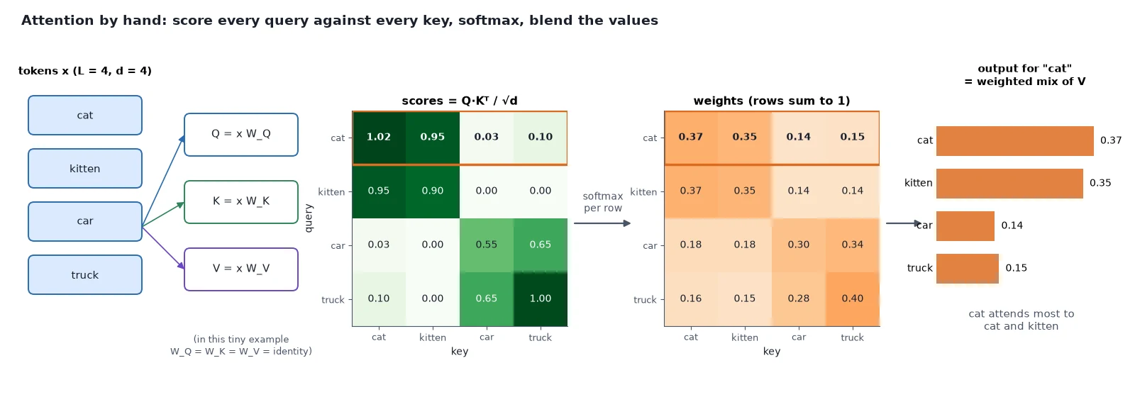
Attention by hand
Before any learned weights, let’s run the formula on four hand-made “word” vectors. To keep it simple we use the embeddings themselves as Q, K and V.
First, the four words and their 4-number embeddings:
import torch

# Four "words" with hand-made 4-number embeddings:
# feature 0 = "is an animal", 1 = "is a cat", 2 = "is a vehicle", 3 = "is big"
words = ["cat", "kitten", "car", "truck"]
x = torch.tensor([[1.0, 1.0, 0.0, 0.2],
                  [1.0, 0.9, 0.0, 0.0],
                  [0.0, 0.0, 1.0, 0.3],
[0.0, 0.0, 1.0, 1.0]]) # (L=4 tokens, d=4)Then the formula itself, three lines of tensor math:
q, k, v = x, x, x                                   # no learned weights yet
d = q.shape[-1]
scores = q @ k.T / d ** 0.5                         # (4, 4): how well each query matches each key
weights = scores.softmax(dim=-1)                    # each row sums to 1
out = weights @ v # (4, 4): weighted mix of valuesFinally, print the scores, the weights, and each word’s top two picks:
torch.set_printoptions(precision=2)
print("scores:\n", scores)
print("weights:\n", weights)
print("row sums:", weights.sum(-1))
for w, row in zip(words, weights):
    best = row.argsort(descending=True)[:2].tolist()
print(f"{w:>6} attends most to: {[words[i] for i in best]}")scores:
tensor([[1.02, 0.95, 0.03, 0.10],
[0.95, 0.90, 0.00, 0.00],
[0.03, 0.00, 0.55, 0.65],
[0.10, 0.00, 0.65, 1.00]])
weights:
tensor([[0.37, 0.35, 0.14, 0.15],
[0.37, 0.35, 0.14, 0.14],
[0.18, 0.18, 0.30, 0.34],
[0.16, 0.15, 0.28, 0.40]])
row sums: tensor([1.00, 1.00, 1.00, 1.00])
cat attends most to: ['cat', 'kitten']
kitten attends most to: ['cat', 'kitten']
car attends most to: ['truck', 'car']
truck attends most to: ['truck', 'car']The animal words pick each other and the vehicle words pick each other. Their vectors point in similar directions, so their dot products are larger.
In a real model, nn.Linear layers learn the W_Q, W_K and W_V projections, so the model can decide what “similar” means for the job at hand.
Attention (scaled dot-product): what, why, how
What it is: a layer that produces, for each token, a weighted mix of all tokens’ values. The weights come from how well that token’s query matches each key.
Why it works: the weights are computed from the data, so the routing changes with every input. A patch of sky can pull information from other sky patches in one image and from a horizon line in another. A fixed filter can’t do that, and it only sees a small neighborhood, while attention sees the whole image in one layer.
How it works: project tokens to Q, K, V with Linear layers. Compute QK^\top / \sqrt{d}, softmax each row, multiply by V. In code: scores = q @ k.transpose(-2, -1) / math.sqrt(d), weights = scores.softmax(-1), out = weights @ v.
Why it works: Every step (matrix multiply, scale, softmax, matrix multiply) is differentiable, so autograd can learn W_Q, W_K and W_V. Step 4 shows this happening.
Watch out: The cost grows with L^2. That is one reason TinyDiT uses 64 patch tokens instead of 1,024 pixel tokens.
What you just built: You ran the attention formula by hand: scores from dot products, weights from a row softmax, and outputs as weighted mixes of values.
Step 2/5: Multi-Head Attention
In this step: We split attention into several heads that look for different things in parallel, and package it as the MultiHeadAttention module TinyDiT uses.
One attention map can only express one notion of “relevant”. Multi-head attention runs several smaller attentions in parallel. With D = 256 and 4 heads, each head works in 256 / 4 = 64 dimensions.
One head might learn “patches with similar color”, another “the patch directly above me”. Their outputs are concatenated back to 256 features and mixed by one more Linear layer:
\begin{gathered} \text{MHA}(X) = \underbrace{\big[\,\text{head}_1 \,\|\, \text{head}_2 \,\|\, \cdots \,\|\, \text{head}_h\,\big]}_{\text{concatenate: } h \times d_{\text{head}} = D}\, \underbrace{W_O}_{\texttt{proj}} \\ \text{head}_i = \text{Attention}(X W_Q^{(i)},\, X W_K^{(i)},\, X W_V^{(i)}) \end{gathered}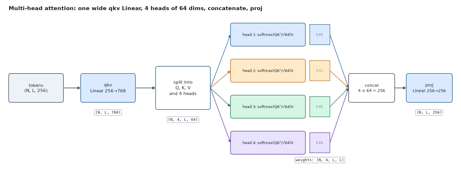
The module, piece by piece
The module lives in tinydit/attention.py. It starts with the attention formula as a plain function:
"""Multi-head self-attention (post 6)."""
import math

import torch
import torch.nn.functional as F
from torch import nn


def attention(q: torch.Tensor, k: torch.Tensor, v: torch.Tensor) -> tuple[torch.Tensor, torch.Tensor]:
    """softmax(q k^T / sqrt(d)) v, written out by hand.

    q, k, v: (..., L, d).  Returns (out (..., L, d), weights (..., L, L)).
    """
    d = q.shape[-1]
    scores = q @ k.transpose(-2, -1) / math.sqrt(d)   # (..., L, L)
    weights = scores.softmax(dim=-1)                   # each row sums to 1
return weights @ v, weightsThe constructor holds the one trick: instead of three separate Linears for Q, K and V, a single nn.Linear(dim, 3 * dim) computes all three in one matrix multiply, which is faster.
class MultiHeadAttention(nn.Module):
    """(N, L, dim) -> (N, L, dim). dim must be divisible by num_heads.

    use_sdpa=False runs the hand-written formula above (and can return the weights).
    use_sdpa=True calls F.scaled_dot_product_attention (post 10), same math, fused kernel.
    """

    def __init__(self, dim: int, num_heads: int, qkv_bias: bool = True, use_sdpa: bool = False):
        super().__init__()
        assert dim % num_heads == 0, "dim must be divisible by num_heads"
        self.num_heads = num_heads
        self.head_dim = dim // num_heads
        self.qkv = nn.Linear(dim, 3 * dim, bias=qkv_bias)   # Q, K, V in one matmul
        self.proj = nn.Linear(dim, dim)                      # mixes the heads back together
self.use_sdpa = use_sdpasplit_heads uses reshape and permute to split the result into Q, K and V and into heads, using exactly the tensor skills from post 2:
    def split_heads(self, x: torch.Tensor) -> tuple[torch.Tensor, torch.Tensor, torch.Tensor]:
        """(N, L, dim) -> q, k, v each (N, heads, L, head_dim)."""
        n, l, _ = x.shape
        qkv = self.qkv(x).reshape(n, l, 3, self.num_heads, self.head_dim)
        q, k, v = qkv.permute(2, 0, 3, 1, 4)     # (3, N, heads, L, head_dim) -> unpack
return q, k, vforward runs attention per head, then concatenates the heads and mixes them with proj:
    def forward(self, x: torch.Tensor, return_weights: bool = False):
        n, l, dim = x.shape
        q, k, v = self.split_heads(x)
        if self.use_sdpa and not return_weights:
            out, weights = F.scaled_dot_product_attention(q, k, v), None
        else:
            out, weights = attention(q, k, v)            # (N, heads, L, head_dim)
        out = out.transpose(1, 2).reshape(n, l, dim)     # concatenate heads
        out = self.proj(out)
return (out, weights) if return_weights else outTrace the shapes
Let’s trace the shapes for a batch of 2 images with 64 tokens each, the size TinyDiT will use:
import torch
from tinydit.attention import MultiHeadAttention

torch.manual_seed(0)
x = torch.randn(2, 64, 256)                     # (N, L, D): 2 images, 64 patch tokens, 256 features
mha = MultiHeadAttention(dim=256, num_heads=4)

qkv = mha.qkv(x)
print("qkv:      ", tuple(qkv.shape))           # one Linear makes Q, K and V together
q, k, v = mha.split_heads(x)
print("q, k, v:  ", tuple(q.shape))             # (N, heads, L, head_dim)
out, w = mha(x, return_weights=True)
print("weights:  ", tuple(w.shape))             # one L x L map per head
print("output:   ", tuple(out.shape))           # same shape as the input
print("rows sum to 1:", torch.allclose(w.sum(-1), torch.ones(2, 4, 64)))
print("untrained weights are almost uniform: mean", round(w.mean().item(), 4),
"| max", round(w.max().item(), 4), "| 1/L =", round(1 / 64, 4))qkv: (2, 64, 768)
q, k, v: (2, 4, 64, 64)
weights: (2, 4, 64, 64)
output: (2, 64, 256)
rows sum to 1: True
untrained weights are almost uniform: mean 0.0156 | max 0.0754 | 1/L = 0.0156Before training, the attention weights are almost uniform. Every token gives every other token roughly 1/64 of its attention, because the model has not learned what to look for yet.
Multi-head attention: what, why, how
What it is: several attention patterns running in parallel, then combined.
Why it works: each head has its own Q, K, V projections, so heads can specialize in different relationships at the same time. Splitting D into h heads of size D/h keeps the total cost about the same as one big head.
How it works: one nn.Linear(D, 3D) makes Q, K and V. reshape(N, L, 3, h, D/h) and permute split them into heads of shape (N, h, L, D/h), attention runs per head, transpose and reshape concatenate the heads back to (N, L, D), and the proj Linear mixes them.
What you just built: A MultiHeadAttention module that maps (N, L, 256) to (N, L, 256) with 4 heads of 64 dimensions, and can return its attention weights for plotting.
Step 3/5: Same Math, Faster Kernel: F.scaled_dot_product_attention
In this step: We check that PyTorch’s fused attention function gives the same answer as our hand-written formula.
PyTorch ships the same formula as one fused function, torch.nn.functional.scaled_dot_product_attention (SDPA). On a GPU it can dispatch to FlashAttention-style kernels that never build the full L \times L table in memory.
Let’s check it really is the same math:
import torch
import torch.nn.functional as F
from tinydit.attention import attention

torch.manual_seed(0)
q, k, v = torch.randn(3, 2, 4, 64, 64).unbind(0)    # (N, heads, L, head_dim) each

ours, _ = attention(q, k, v)
fused = F.scaled_dot_product_attention(q, k, v)     # PyTorch's built-in kernel
print("max difference:", (ours - fused).abs().max().item())
print("same result:", torch.allclose(ours, fused, atol=1e-5))max difference: 5.364418029785156e-07
same result: TrueThe tiny difference is floating-point rounding.
Note: Our module keeps the hand-written path by default, because it can return the weights for plotting. The use_sdpa=True flag switches to the fused kernel, and post 10 turns it on for speed.
What you just built: Proof that F.scaled_dot_product_attention and our attention() agree to within rounding, plus a use_sdpa switch you will flip in post 10.
Step 4/5: Watch Attention Learn
In this step: We train a single attention layer on a task with an obvious answer and look at the attention map it learns.
Uniform weights are boring. Let’s give a single attention layer a job where the right answer is obvious: every position must output the biggest number in its sequence. The only way to do that is for every query to put its weight on the max token.
The model embeds each number as a token, runs one attention head, and reads a number back out:
"""Train one attention layer to find the biggest number in a sequence, then look at its weights."""
import torch
from torch import nn
from tinydit.attention import MultiHeadAttention

torch.manual_seed(0)
L, D = 8, 32

class FindMax(nn.Module):
    def __init__(self):
        super().__init__()
        self.embed = nn.Linear(1, D)                      # number -> token vector
        self.attn = MultiHeadAttention(D, num_heads=1)
        self.readout = nn.Linear(D, 1)                    # token vector -> number

    def forward(self, nums, return_weights=False):
        tok = self.embed(nums.unsqueeze(-1))              # (N, L) -> (N, L, D)
        mixed, w = self.attn(tok, return_weights=True)
        out = self.readout(mixed).squeeze(-1)             # (N, L)
return (out, w) if return_weights else outTraining is the usual loop from post 5, on random sequences whose target is the sequence max:
model = FindMax()
opt = torch.optim.AdamW(model.parameters(), lr=3e-3)
for step in range(1501):
    nums = torch.rand(256, L)                             # random sequences
    target = nums.max(dim=1, keepdim=True).values.expand(-1, L)  # every position should output the max
    loss = ((model(nums) - target) ** 2).mean()
    opt.zero_grad(); loss.backward(); opt.step()
    if step % 500 == 0:
print(f"step {step:4d} | loss {loss.item():.5f}")Then we feed one fixed sequence and print the learned attention weights:
seq = torch.tensor([[0.10, 0.50, 0.20, 0.95, 0.30, 0.05, 0.60, 0.40]])
with torch.no_grad():
    pred, w = model(seq, return_weights=True)
torch.set_printoptions(precision=2, sci_mode=False)
print("input   :", seq[0])
print("predicted:", pred[0])
print("attention weights (row = query position, col = key position):")
print(w[0, 0])
print("each row's favourite position:", w[0, 0].argmax(-1).tolist(), "(the 0.95 is at position 3)")step 0 | loss 0.81119
step 500 | loss 0.00006
step 1000 | loss 0.00002
step 1500 | loss 0.00001
input : tensor([0.10, 0.50, 0.20, 0.95, 0.30, 0.05, 0.60, 0.40])
predicted: tensor([0.95, 0.95, 0.95, 0.95, 0.95, 0.95, 0.95, 0.95])
attention weights (row = query position, col = key position):
tensor([[0.00, 0.00, 0.00, 1.00, 0.00, 0.00, 0.00, 0.00],
[0.00, 0.00, 0.00, 1.00, 0.00, 0.00, 0.00, 0.00],
[0.00, 0.00, 0.00, 1.00, 0.00, 0.00, 0.00, 0.00],
[0.00, 0.00, 0.00, 1.00, 0.00, 0.00, 0.00, 0.00],
[0.00, 0.00, 0.00, 1.00, 0.00, 0.00, 0.00, 0.00],
[0.00, 0.00, 0.00, 1.00, 0.00, 0.00, 0.00, 0.00],
[0.00, 0.00, 0.00, 1.00, 0.00, 0.00, 0.00, 0.00],
[0.00, 0.00, 0.00, 1.00, 0.00, 0.00, 0.00, 0.00]])
each row's favourite position: [3, 3, 3, 3, 3, 3, 3, 3] (the 0.95 is at position 3)Every row put essentially 100% of its weight on position 3, where the 0.95 lives.
Nobody told the model “find the maximum”. Gradient descent shaped W_Q and W_K until the largest number produces the largest score for every query. This is what we mean by learned importance.
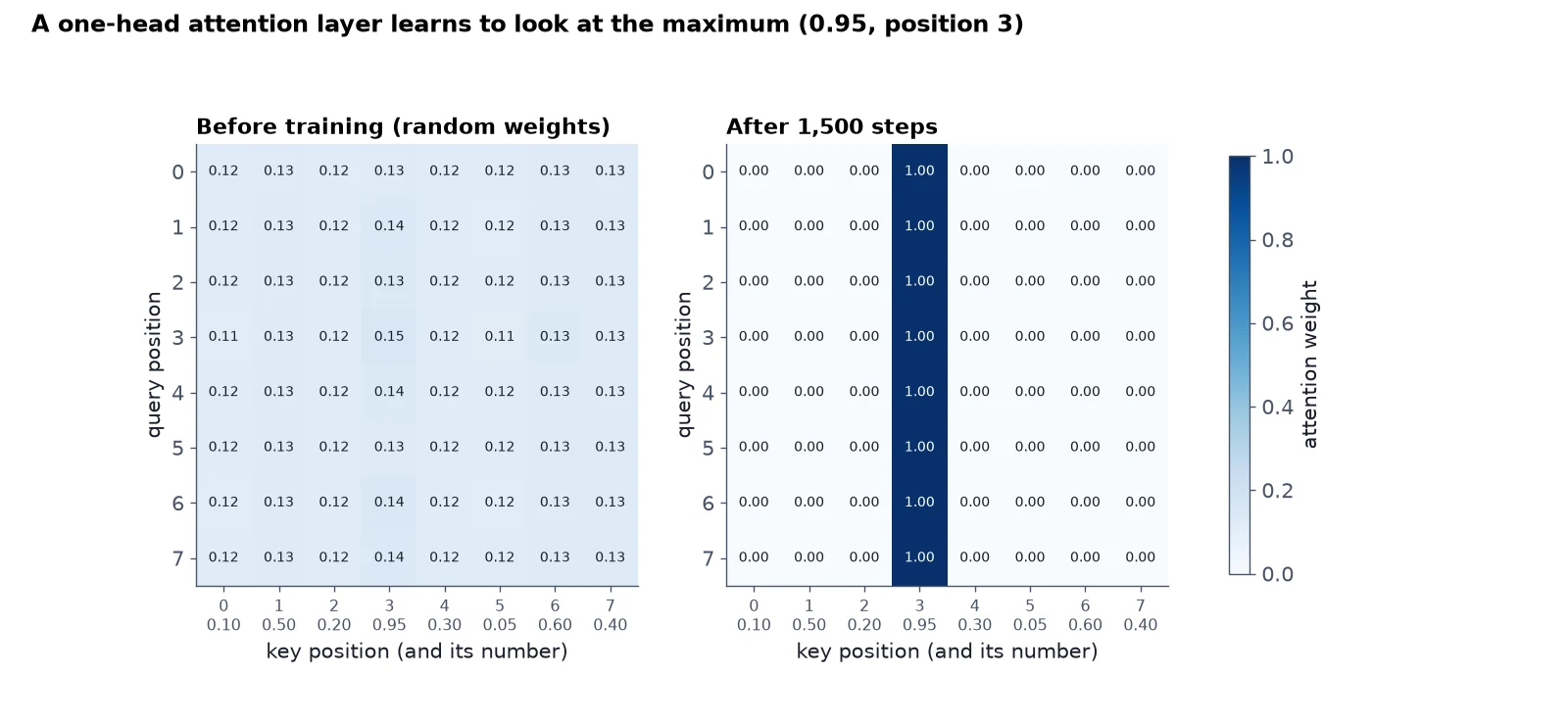
What you just built: A trained one-head attention layer whose attention map points every query at the max token.
Step 5/5: The Transformer Block
In this step: We wrap attention and the feed-forward network from post 5 into the pre-norm TransformerBlock, the repeatable unit of TinyDiT.
Attention mixes information between tokens. The feed-forward network from post 5 processes each token on its own.
A transformer block alternates the two, each wrapped in a LayerNorm and a residual connection. We use the pre-norm arrangement: normalize first, then the sub-layer, then add the input back.
\begin{gathered} \underbrace{x \leftarrow x + \operatorname{Attn}\big(\operatorname{LN}_1(x)\big)}_{\text{tokens talk to each other}} \\ \underbrace{x \leftarrow x + \operatorname{FFN}\big(\operatorname{LN}_2(x)\big)}_{\text{each token thinks on its own}} \end{gathered}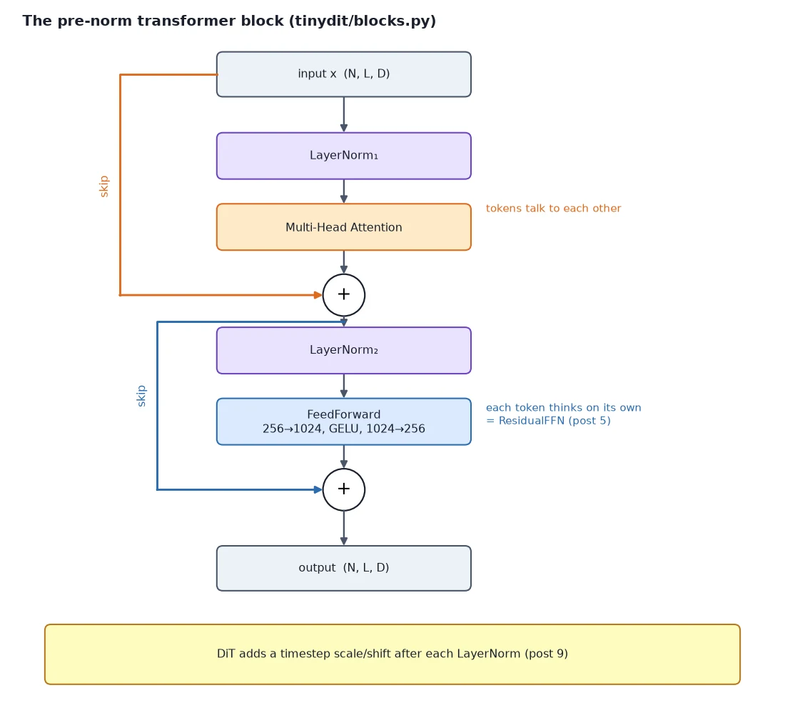
The second line is exactly the ResidualFFN we built in post 5, so the block is short. This is tinydit/blocks.py:
"""The pre-norm transformer block TinyDiT stacks (post 6)."""
import torch
from torch import nn

from .attention import MultiHeadAttention
from .layers import ResidualFFN


class TransformerBlock(nn.Module):
    """x = x + Attn(LN(x));  x = x + FFN(LN(x)).   (N, L, dim) -> (N, L, dim)."""

    def __init__(self, dim: int, num_heads: int, mlp_ratio: float = 4.0, use_sdpa: bool = False):
        super().__init__()
        self.norm1 = nn.LayerNorm(dim)
        self.attn = MultiHeadAttention(dim, num_heads, use_sdpa=use_sdpa)
        self.ffn = ResidualFFN(dim, mlp_ratio)   # holds its own LayerNorm (ffn.norm) and residual

    def forward(self, x: torch.Tensor) -> torch.Tensor:
        x = x + self.attn(self.norm1(x))
        x = self.ffn(x)
return xNow build one block and count its parameters:
import torch
from tinydit.blocks import TransformerBlock

torch.manual_seed(0)
block = TransformerBlock(dim=256, num_heads=4)
x = torch.randn(2, 64, 256)
y = block(x)
print("in :", tuple(x.shape))
print("out:", tuple(y.shape))

for name, module in block.named_children():
    n = sum(p.numel() for p in module.parameters())
    print(f"  {name:6s} {n:9,d} params")
print(f"  total  {sum(p.numel() for p in block.parameters()):9,d} params")

# Stack six of them, like TinyDiT will:
stack = torch.nn.Sequential(*[TransformerBlock(256, 4) for _ in range(6)])
print("6 blocks:", tuple(stack(x).shape), f"{sum(p.numel() for p in stack.parameters()):,} params")in : (2, 64, 256)
out: (2, 64, 256)
norm1 512 params
attn 263,168 params
ffn 526,080 params
total 789,760 params
6 blocks: (2, 64, 256) 4,738,560 paramsThe block takes (N, L, D) and returns (N, L, D). Same shape in, same shape out is what makes it stackable: TinyDiT’s whole backbone is this block repeated six times, about 4.7 million parameters.
Note: Two-thirds of each block’s parameters live in the feed-forward network, not in attention.
TransformerBlock: what, why, how
What it is: the repeatable unit of TinyDiT: one round of “tokens talk” (attention) followed by one round of “each token thinks” (feed-forward).
Why it works: depth comes from stacking one well-understood block. Residual connections let each block make a small correction instead of rebuilding the representation, and give gradients a direct path back to the early layers. Pre-norm LayerNorm keeps the inputs to each sub-layer on a stable scale, whatever the residual stream has grown to.
How it works: x = x + attn(norm1(x)), then x = x + mlp(norm2(x)) (inside ResidualFFN). Shapes stay (N, L, D) throughout, so nn.Sequential(*[TransformerBlock(256, 4) for _ in range(6)]) just works.
Why it works: Pre-norm is the arrangement DiT and most modern transformers use. The residual path stays a clean “highway” from input to output that the normalization never touches, which makes deep stacks easier to train than the original 2017 post-norm layout.
Note: In post 9 the LayerNorms gain a timestep-dependent scale and shift (adaptive LayerNorm), which is how DiT tells every block how noisy its input is.
What you just built: The pre-norm TransformerBlock: LN → attention → residual, then LN → FFN → residual, mapping (N, L, D) to (N, L, D).
Recap
- PyTorch attention computes \operatorname{softmax}(QK^\top/\sqrt{d})\,V: scores from queries and keys, weights from softmax, output as a weighted mix of values.
- Multi-head attention splits D into heads that attend in parallel, then concatenates and projects them. Our module uses one fused
qkvLinear. F.scaled_dot_product_attentiongives the same result (difference about 5 \times 10^{-7}) with a faster kernel. We’ll switch to it in post 10.- A single attention layer learned to put 100% of its weight on the max token, which is learned importance in action.
- The pre-norm
TransformerBlockmaps(N, L, D)to(N, L, D). Six of them form TinyDiT’s 4.7M-parameter backbone.
Next up: There’s one problem: our block eats a sequence of tokens, but CIFAR-10 gives us images. In Patch Embeddings in PyTorch: How a Transformer Reads an Image we cut images into patches, turn them into tokens, tell the model where each patch sits, and fold tokens back into an image.
Series: PyTorch Tutorial 2026 (14 posts)
- Post 1: PyTorch Tutorial 2026: From Tensors to Tiny Diffusion
- Post 2: PyTorch Tensors Explained: Shapes, Broadcasting, and Images as Arrays
- Post 3: PyTorch Autograd: How backward() Builds Gradients
- Post 4: PyTorch DataLoader Explained: Datasets, Batches, and Image Folders
- Post 5: PyTorch nn.Module and the Training Loop: Layers, Loss, and Checkpoints
- Post 6: Attention and the Transformer Block in PyTorch (you are here)
- Post 7: Patch Embeddings in PyTorch: How a Transformer Reads an Image
- Post 8: Flow Matching in PyTorch: Train a Model to Follow a Straight Line
- Post 9: Build a Tiny Diffusion Transformer in PyTorch (DiT from Scratch)
- Post 10: torch.compile, Mixed Precision, and SDPA: Speed Up TinyDiT
- Post 11: RMSNorm, QK-Norm, SwiGLU, and 2D RoPE in a Tiny DiT
- Post 12: adaLN-Zero and Classifier-Free Guidance in PyTorch
- Post 13: MMDiT Joint Attention in PyTorch: Two Streams, One Generator
- Post 14: Train and Sample Like 2026: Logit-Normal Steps, EMA, and Few-Step Flow
← Previous: Post 5: PyTorch nn.Module and the Training Loop: Layers, Loss, and Checkpoints
Next → Post 7: Patch Embeddings in PyTorch: How a Transformer Reads an Image