Train and Sample Like 2026: Logit-Normal Steps, EMA, and Few-Step Flow
Where you are: Post 14 of 14 in PyTorch Tutorial 2026 · about 14 min read
What you’ll build: Logit-normal timestep sampling, an EMA copy of the weights, and reflow for 1- and 2-step sampling, each measured on TinyDiT, then a side-by-side of every stage of the series.
You’ll need: Post 8 (flow matching, euler_sample), Post 11 (2D RoPE, QK-norm) and Post 12 (adaLN-Zero, guidance).
In this post:
- Introduction
- Step 1/6: Logit-Normal Timesteps: Train Where It's Hard
- Step 2/6: EMA: Sample from an Average of the Weights
- Step 3/6: Before/After: Logit-Normal and EMA on TinyDiT
- Step 4/6: Reflow: Straighten the Paths
- Step 5/6: Before/After: Reflow on TinyDiT
- Step 6/6: Simple vs Expert: Where We Started, Where We Ended
- Where to Go Next
- Recap
Series: PyTorch Tutorial 2026 (14 posts)
- Post 1: PyTorch Tutorial 2026: From Tensors to Tiny Diffusion
- Post 2: PyTorch Tensors Explained: Shapes, Broadcasting, and Images as Arrays
- Post 3: PyTorch Autograd: How backward() Builds Gradients
- Post 4: PyTorch DataLoader Explained: Datasets, Batches, and Image Folders
- Post 5: PyTorch nn.Module and the Training Loop: Layers, Loss, and Checkpoints
- Post 6: Attention and the Transformer Block in PyTorch
- Post 7: Patch Embeddings in PyTorch: How a Transformer Reads an Image
- Post 8: Flow Matching in PyTorch: Train a Model to Follow a Straight Line
- Post 9: Build a Tiny Diffusion Transformer in PyTorch (DiT from Scratch)
- Post 10: torch.compile, Mixed Precision, and SDPA: Speed Up TinyDiT
- Post 11: RMSNorm, QK-Norm, SwiGLU, and 2D RoPE in a Tiny DiT
- Post 12: adaLN-Zero and Classifier-Free Guidance in PyTorch
- Post 13: MMDiT Joint Attention in PyTorch: Two Streams, One Generator
- Post 14: Train and Sample Like 2026: Logit-Normal Steps, EMA, and Few-Step Flow (you are here)
Introduction
This is the last post. Our TinyDiT already has a 2026-style block (post 11), class conditioning with guidance (post 12) and joint attention (post 13).
What’s left are three tricks that change how we train and sample, not the architecture:
- logit-normal timestep sampling: spend training time where it matters;
- EMA weights: sample from a smoothed copy of the model;
- reflow: the “rectified” part of rectified flow PyTorch models like SD3, which straightens the paths so that a handful of sampling steps is enough.
As in every Expert post, each one gets a citation and a measured before/after on TinyDiT. Then we put the simple post-9 model and the final model side by side, and look at where to go next.
Note: CPU settings used in this post: the post-12 class-conditional TinyDiT (dim 128, depth 4, 4 heads, adaLN-Zero) with 2D RoPE and QK-norm from post 11, batch 128, 3,000 steps, 8-core CPU. Reflow: 20,000 teacher pairs and 2,000 fine-tuning steps. Scores on 1,000 samples (100 per class).
Step 1/6: Logit-Normal Timesteps: Train Where It’s Hard
In this step: We change how the training time t is drawn, so more training steps land on the middle noise levels.
Until now we picked the training time t uniformly between 0 and 1. But not all times are equally useful to practise.
Near t = 1 the input is pure noise and the best answer is “the average image”, which is easy. Near t = 0 the input is almost clean and the answer is a tiny correction, also easy. The hard, informative part is in the middle, where the model must decide what the image will be.
SD3 (Esser et al., 2024) tested many timestep distributions for rectified flow and found that logit-normal sampling, which puts more training steps in the middle, gave the best results:
\begin{gathered} t = \operatorname{sigmoid}(u), \\ u \sim \mathcal{N}(m, s^2) \\ (\text{we use } m = 0,\ s = 1) \end{gathered}def sample_t(n: int, device=None, dist: str = "uniform", mean: float = 0.0, std: float = 1.0,
generator: torch.Generator | None = None) -> torch.Tensor:
"""Training times. 'uniform': U(0, 1). 'logit_normal': sigmoid(N(mean, std)) as in SD3 (post 14)."""
if dist == "uniform":
return torch.rand(n, device=device, generator=generator)
if dist == "logit_normal":
return torch.sigmoid(mean + std * torch.randn(n, device=device, generator=generator))
raise ValueError(f"unknown t distribution {dist!r}")A quick count of where the samples land:
import torch
from tinydit.flow import sample_t

torch.manual_seed(0)
bins = torch.linspace(0, 1, 11)
for dist in ["uniform", "logit_normal"]:
    t = sample_t(100_000, dist=dist)
    counts = torch.histc(t, bins=10, min=0, max=1) / len(t)
    bar = " ".join(f"{c:.2f}" for c in counts)
print(f"{dist:12s} share of t in each tenth [0-0.1 ... 0.9-1]: {bar}")uniform share of t in each tenth [0-0.1 ... 0.9-1]: 0.10 0.10 0.10 0.10 0.10 0.10 0.10 0.10 0.10 0.10
logit_normal share of t in each tenth [0-0.1 ... 0.9-1]: 0.01 0.07 0.12 0.14 0.16 0.16 0.14 0.11 0.07 0.01Uniform sampling gives every tenth of the range 10% of the training steps. Logit-normal gives the middle tenths 14 to 16% each and the two ends only 1% each. In train.py it’s one flag: --t-dist logit_normal.
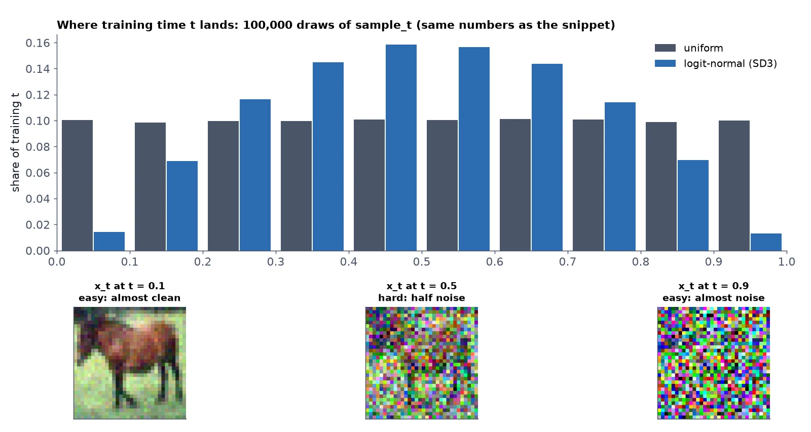
Logit-normal timestep sampling: what, why, how
What it is: a way of choosing which noise levels to train on.
Why it works: the middle noise levels are the hardest and most informative, so giving them more training steps improved large latent models for the same budget (SD3, 2024). On TinyDiT it made probe-FD worse (Step 3), so we measure it but don’t keep it.
How it works: t = sigmoid(m + s * randn(n)) instead of rand(n). In TinyDiT: --t-dist logit_normal.
What you just built: sample_t with a logit-normal option, behind the --t-dist logit_normal flag.
Step 2/6: EMA: Sample from an Average of the Weights
In this step: We keep a slowly moving average of the weights and sample from it instead of the raw weights.
During training, the weights jump around a little with every noisy minibatch. An exponential moving average (EMA) keeps a second copy that follows the real weights slowly:
\begin{gathered} \theta_{\text{EMA}} \leftarrow d \cdot \theta_{\text{EMA}} + (1 - d) \cdot \theta \\ d = \min\!\Big(0.999,\ \frac{1 + n}{10 + n}\Big) \end{gathered}We train the normal model, but sample from the EMA copy. Almost every diffusion model since DDPM does this (DiT uses d = 0.9999 over hundreds of thousands of steps; for our 3,000 steps, 0.999 is the right scale).
Why it works: The warm-up formula for d stops the EMA from remembering the random starting weights for too long.
class EMA:
    """ema = decay * ema + (1 - decay) * weights, after every optimizer step.

    The effective decay ramps up as min(decay, (1 + step) / (10 + step)), so early on the
    average is not stuck near the random initial weights.
    """

    def __init__(self, model: nn.Module, decay: float = 0.999):
        self.decay = decay
        self.model = copy.deepcopy(model).eval().requires_grad_(False)
        self.updates = 0

    @torch.no_grad()
    def update(self, model: nn.Module) -> None:
        self.updates += 1
        d = min(self.decay, (1 + self.updates) / (10 + self.updates))
        for e, p in zip(self.model.parameters(), model.parameters()):
            e.lerp_(p.detach(), 1 - d)                 # e += (1 - d) * (p - e)
        for e, b in zip(self.model.buffers(), model.buffers()):
e.copy_(b)A toy weight that bounces around a true centre of 1.00:
import torch
from torch import nn
from tinydit.ema import EMA

model = nn.Linear(1, 1, bias=False)
nn.init.zeros_(model.weight)
ema = EMA(model, decay=0.999)
torch.manual_seed(0)
for step in range(1, 3001):
    with torch.no_grad():
        model.weight.fill_(1.0 + 0.3 * torch.randn(()))   # noisy training weights around 1.0
    ema.update(model)
    if step in (1, 10, 100, 1000, 3000):
        print(f"step {step:4d}: decay used {min(0.999, (1 + step) / (10 + step)):.3f} | raw weight {model.weight.item():+.3f} | "
f"EMA weight {ema.model.weight.item():+.3f}")step 1: decay used 0.182 | raw weight +1.462 | EMA weight +1.196
step 10: decay used 0.550 | raw weight +0.879 | EMA weight +0.912
step 100: decay used 0.918 | raw weight +0.637 | EMA weight +0.941
step 1000: decay used 0.991 | raw weight +1.523 | EMA weight +1.004
step 3000: decay used 0.997 | raw weight +1.186 | EMA weight +0.995The raw weight bounces between 0.64 and 1.52, while the EMA weight settles near the true centre (1.00). EMATrainer calls ema.update(model) after every optimizer step and saves the EMA weights in the checkpoint under "ema". In train.py: --ema 0.999.
EMA weights: what, why, how
What it is: a smoother copy of the model to sample from.
Why it works: averaging over recent weights cancels some of the noise from individual minibatch updates. Used by almost every diffusion model since DDPM (Ho et al., 2020) and DiT.
How it works: after each optimizer step, ema = lerp(ema, weights, 1 - d); sample with the EMA copy. In TinyDiT: --ema 0.999.
What you just built: An EMA class with warm-up, updated after every optimizer step and saved under "ema" in the checkpoint.
Step 3/6: Before/After: Logit-Normal and EMA on TinyDiT
In this step: We score both tricks from one pair of training runs: uniform vs logit-normal t, each with raw and EMA weights.
Two runs, identical except for the timestep distribution: the post-12 adaLN-Zero model (uniform t) and the same model trained with logit-normal t.
Both runs kept an EMA copy, so each one gives us two models to score: the raw trained weights and the EMA weights. That’s both before/afters from one pair of runs:
import json
from pathlib import Path

def load(name):
    return json.loads(Path(f"../runs/{name}/metrics.json").read_text())

uni, logn = load("p12_cond_zero"), load("p14_lognorm_ema")    # identical except the t distribution
print(f"{'run':30s} {'val MSE':>8s} {'FD w=1.5':>9s} {'acc w=1.5':>10s} {'FD w=3':>7s} {'acc w=3':>8s}")
for name, m in [("uniform t", uni), ("logit-normal t", logn)]:
    for kind in ("raw", "ema"):
        r = m[kind]
        label = f"{name}, {'EMA weights' if kind == 'ema' else 'raw weights'}"
        print(f"{label:30s} {r['val_mse']:8.4f} {r['cfg1.5']['probe_fd']:9.1f} {r['cfg1.5']['probe_acc']:10.1%} "
f"{r['cfg3.0']['probe_fd']:7.1f} {r['cfg3.0']['probe_acc']:8.1%}")run val MSE FD w=1.5 acc w=1.5 FD w=3 acc w=3
uniform t, raw weights 0.2157 50.3 32.7% 52.3 45.2%
uniform t, EMA weights 0.2132 47.1 36.2% 48.0 50.1%
logit-normal t, raw weights 0.2255 54.6 34.3% 52.9 47.3%
logit-normal t, EMA weights 0.2243 52.6 34.2% 50.0 49.5%| Run | Val MSE | Probe-FD (w = 1.5) | Class acc (w = 1.5) | Probe-FD (w = 3) | Class acc (w = 3) |
|---|---|---|---|---|---|
| Uniform t, raw weights | 0.2157 | 50.3 | 32.7% | 52.3 | 45.2% |
| Uniform t, EMA weights | 0.2132 | 47.1 | 36.2% | 48.0 | 50.1% |
| Logit-normal t, raw weights | 0.2255 | 54.6 | 34.3% | 52.9 | 47.3% |
| Logit-normal t, EMA weights | 0.2243 | 52.6 | 34.2% | 50.0 | 49.5% |
What the numbers say:
- EMA is a free, clear win. In both runs the EMA copy beat the raw weights on almost every score: val MSE, probe-FD and class accuracy. It costs one extra copy of the weights in memory and nothing at all in training quality. Keep it on.
- Logit-normal timesteps did not help TinyDiT. The probe-FD got worse (54.6 vs 50.3 with raw weights, 52.6 vs 47.1 with EMA), and class accuracy only moved a little.
Watch out: The val MSE also got worse with logit-normal, but that one isn’t a fair judge here: it tests at uniformly random times, so it rewards the uniform model for practising the times it’s tested on.
Why the difference from SD3?
SD3 trained large models on high-resolution latents for hundreds of thousands of steps. Our model works on 32×32 pixels for 3,000 steps, and with logit-normal sampling only about 1% of training steps land near t = 0, where the sampler adds the last fine details. At this size and budget those ends seem to matter more than the paper’s setting suggests.
It’s one seed per setting, but the probe-FD gap is large. So the honest verdict for TinyDiT is: logit-normal is a good default for big latent models, and not worth it here.
Note: If you want to try a middle ground, SD3 also tested heavier-tailed variants, and sample_t takes mean and std so you can widen the bell (for example std=1.5).
What you just built: A measured verdict: EMA improves probe-FD from 50.3 to 47.1 and class accuracy from 32.7% to 36.2% at w = 1.5; logit-normal makes probe-FD worse (54.6 vs 50.3), so we drop it.
Step 4/6: Reflow: Straighten the Paths
In this step: We fine-tune a student on the teacher’s own noise-to-image pairs, so its paths become straight enough for 1 or 2 sampling steps.
In Flow Matching in PyTorch: Train a Model to Follow a Straight Line we saw that flow-matching paths are straight for each training pair, but the model’s actual paths bend, because noise and images were paired at random and the lines cross. That’s why one or two Euler steps give blurry results.
Reflow (Liu et al., Flow Straight and Fast: Learning to Generate and Transfer Data with Rectified Flow, ICLR 2023) fixes this in three steps:
- Use the trained model (the “teacher”) to turn fixed noise x_1 into an image x_0, with many steps.
- Train a copy (the “student”) with the same flow-matching loss, but on those fixed pairs (x_0, x_1) instead of random ones.
- The teacher’s paths don’t cross (it’s a deterministic map), so the student learns nearly straight paths, and Euler with few steps follows them much better.
The loss is the post-8 straight-line loss, on fixed pairs:
class ReflowLoss:
    """Rectified-flow "reflow" (Liu et al., 2022), post 14. batch = (x0, x1, y): a FIXED pair made by the teacher,
    x1 = noise, x0 = the teacher's sample from that noise. Same straight-line loss, but the pairing is no longer random,
    so the lines stop crossing and few-step sampling gets more accurate."""

    def __init__(self, conditional: bool = True):
        self.conditional = conditional

    def __call__(self, model: nn.Module, batch) -> torch.Tensor:
        x0, x1, y = batch
        t = sample_t(x0.shape[0], x0.device)
        xt = interpolate(x0, x1, t)
        pred = model(xt, t, y) if self.conditional else model(xt, t)
return F.mse_loss(pred, x1 - x0)Why it works: Our teacher samples with CFG, so the guidance gets “baked in”: the student samples without CFG, which halves the work per step on top of needing fewer steps.
The full script is code/reflow.py. First, the teacher turns fixed noise into images, with CFG:
@torch.no_grad()
def make_pairs(teacher, n, steps, cfg_scale, seed=123, batch=250):
    g = torch.Generator().manual_seed(seed)
    noise = torch.randn(n, 3, 32, 32, generator=g)
    labels = torch.randint(0, 10, (n,), generator=g)
    images = torch.cat([euler_sample(teacher, noise[i:i + batch], steps, y=labels[i:i + batch], cfg_scale=cfg_scale,
                                     null_class=10) for i in range(0, n, batch)])
return images.clamp(-1, 1), noise, labelsThen the student starts as a copy of the teacher (its EMA weights) and fine-tunes on those fixed pairs:
def main(teacher_dir, out, pairs, steps, lr, cfg_scale, teacher_steps, threads, n_eval, work):
    torch.set_num_threads(threads)
    torch.manual_seed(0)
    out = Path(out); out.mkdir(parents=True, exist_ok=True)
    ckpt = torch.load(Path(teacher_dir) / "model.pt", weights_only=False)
    teacher = ExpertTinyDiT(ExpertConfig(**ckpt["config"]))
    teacher.load_state_dict(ckpt["ema"] if "ema" in ckpt else ckpt["model"])
    teacher.eval()

    t0 = time.time()
    x0, x1, y = make_pairs(teacher, pairs, teacher_steps, cfg_scale)
    pair_time = time.time() - t0
    print(f"made {pairs} pairs in {pair_time:.0f}s", flush=True)

    student = copy.deepcopy(teacher)
    trainer = FastTrainer(student, ReflowLoss(), lr=lr)
    loader = DataLoader(TensorDataset(x0, x1, y), batch_size=128, shuffle=True, drop_last=True)
    t0 = time.time()
    while trainer.step < steps:
        for batch in loader:
            loss = trainer.train_step(batch)
            if trainer.step % 250 == 0:
                print(f"[reflow] step {trainer.step} loss {loss:.4f} ({time.time() - t0:.0f}s)", flush=True)
            if trainer.step >= steps:
                break
train_time = time.time() - t0Finally, teacher and student sample the same fresh noise at 1, 2 and 4 steps; the student runs without CFG (w = 1.0):
    probe = load_probe(f"{work}/probe.pt")
    real = torch.load(f"{work}/probe_real_feats.pt", weights_only=True)
    g = torch.Generator().manual_seed(7)                      # fresh eval noise, not used for the pairs
    noise = torch.randn(n_eval, 3, 32, 32, generator=g)
    labels = torch.arange(n_eval) % 10
    ref = sample_all(teacher, noise, labels, teacher_steps, cfg_scale)
    res = {"teacher_20": probe_scores(probe, ref, real, labels)}
    for k in (1, 2, 4):
        for name, model, w in (("teacher", teacher, cfg_scale), ("student", student, 1.0)):
            s = sample_all(model, noise, labels, k, w)
            r = probe_scores(probe, s, real, labels)
            r["mse_to_teacher20"] = round((s - ref).pow(2).mean().item(), 4)
            res[f"{name}_{k}"] = r
            print(name, k, r, flush=True)
            grid = s[:100].reshape(10, 10, 3, 32, 32).transpose(0, 1).reshape(100, 3, 32, 32)
            save_grid(grid, out / f"samples_{name}_{k}step.png", nrow=10)
    metrics = {"teacher": str(teacher_dir), "pairs": pairs, "teacher_steps": teacher_steps, "cfg_scale": cfg_scale,
               "steps": steps, "lr": lr, "pair_time_s": round(pair_time, 1), "train_time_s": round(train_time, 1),
               "results": res}
    (out / "metrics.json").write_text(json.dumps(metrics, indent=1))
    torch.save({"model": student.state_dict(), "config": ckpt["config"]}, out / "model.pt")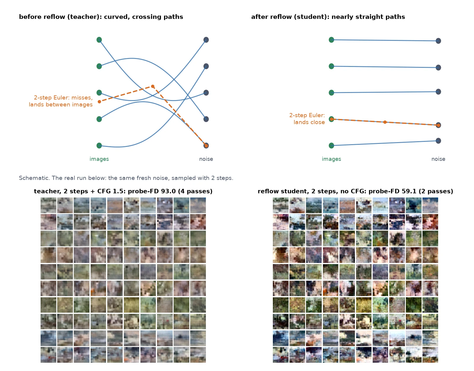
Reflow (ReflowLoss): what, why, how
What it is: a fine-tuning step that gives fewer sampling steps for the same quality.
Why it works: training on the teacher’s own (noise, image) pairs removes crossing paths, so the learned paths become straighter and a big Euler step stays on track (Liu et al., 2023).
How it works: generate pairs with the teacher, then fine-tune a copy with ReflowLoss (the same straight-line loss on fixed pairs). Sample the student with 1 to 4 steps, no CFG.
What you just built: ReflowLoss and code/reflow.py: teacher pairs in, a few-step student out.
Step 5/6: Before/After: Reflow on TinyDiT
In this step: We compare the teacher and the reflow student at 1, 2 and 4 sampling steps.
The teacher is the logit-normal model from Step 3, with its EMA weights. We set up the reflow run before we knew logit-normal wouldn’t win, but that doesn’t matter here: reflow is judged by how well the student matches its own teacher with fewer steps.
The teacher made 20,000 pairs (20 Euler steps, CFG 1.5) in 12 minutes, and the student fine-tuned on them for 2,000 steps in 5 minutes. Then both drew the same 1,000 images from fresh noise at 1, 2 and 4 steps:
import json
from pathlib import Path

m = json.loads(Path("../runs/p14_reflow/metrics.json").read_text())
res = m["results"]
print(f"pairs: {m['pairs']} made in {m['pair_time_s']:.0f}s | reflow fine-tune: {m['steps']} steps in {m['train_time_s']:.0f}s")
t20 = res["teacher_20"]
print(f"reference, teacher 20 steps + CFG {m['cfg_scale']}: probe-FD {t20['probe_fd']:.1f}, class acc {t20['probe_acc']:.1%}")
print(f"\n{'steps':>5s} {'model':8s} {'forward passes':>14s} {'probe-FD':>9s} {'class acc':>9s} {'MSE to 20-step':>15s}")
for k in (1, 2, 4):
    for name, passes in (("teacher", 2 * k), ("student", k)):    # teacher uses CFG: 2 passes per step
        r = res[f"{name}_{k}"]
print(f"{k:5d} {name:8s} {passes:14d} {r['probe_fd']:9.1f} {r['probe_acc']:9.1%} {r['mse_to_teacher20']:15.4f}")pairs: 20000 made in 712s | reflow fine-tune: 2000 steps in 321s
reference, teacher 20 steps + CFG 1.5: probe-FD 52.6, class acc 34.2%
steps model forward passes probe-FD class acc MSE to 20-step
1 teacher 2 208.9 10.0% 0.1640
1 student 1 61.3 29.3% 0.0058
2 teacher 4 93.0 25.6% 0.0605
2 student 2 59.1 31.6% 0.0032
4 teacher 8 62.4 27.5% 0.0253
4 student 4 57.4 32.0% 0.0024| Steps | Teacher (with CFG) probe-FD | Student (no CFG) probe-FD | Teacher class acc | Student class acc | Student forward passes |
|---|---|---|---|---|---|
| 1 | 208.9 | 61.3 | 10.0% | 29.3% | 1 |
| 2 | 93.0 | 59.1 | 25.6% | 31.6% | 2 |
| 4 | 62.4 | 57.4 | 27.5% | 32.0% | 4 |
| 20 (reference) | 52.6 | – | 34.2% | – | (teacher: 40) |
What the numbers say:
- Reflow works, dramatically, at 1 and 2 steps. With one Euler step the teacher produces mush (probe-FD 209, class accuracy at chance), because its paths are curved and one straight jump misses badly. The student, after just 5 minutes of fine-tuning, gets probe-FD 61 in one step.
- Its paths really did become straighter. The “MSE to 20-step” column shows why: the student’s 1-step image is 28× closer to the teacher’s 20-step result than the teacher’s own 1-step image is (0.0058 vs 0.1640).
- At 4 steps the teacher catches up a lot (62.4), and the student’s advantage shrinks to about 5 points. Reflow matters most when you want 1 or 2 steps.
Watch out: It’s not free quality. The student’s 2-step samples (59.1) are still worse than the teacher at 20 steps (52.6), and class accuracy drops from 34.2% to 31.6%. Reflow trades a little quality for a 20× cut in forward passes (2 instead of 40, since the student also doesn’t need CFG).
What you just built: A reflow student: one-step probe-FD 208.9 → 61.3 and two-step 93.0 → 59.1, with one forward pass per step.
Step 6/6: Simple vs Expert: Where We Started, Where We Ended
In this step: We put every stage of the series in one table and read off what helped and what didn’t.
Here’s every stage of the series in one table, read from the same metrics.json files.
Watch out: Each row is its own training run, not a stack of everything before it, and the first two rows are unconditional, so compare probe-FD within the same kind of model.
import json
from pathlib import Path

def load(name):
    return json.loads(Path(f"../runs/{name}/metrics.json").read_text())

rows = [("post 9 TinyDiT, unconditional", "p11_base_s0", "raw", None),
        ("post 11 block, unconditional", "p11_all", "raw", None),
        ("post 12 adaLN-Zero + labels", "p12_cond_zero", "raw", "1.5"),
        ("post 12 model, EMA weights", "p12_cond_zero", "ema", "1.5"),
        ("post 13 joint attention", "p13_joint22", "raw", "1.5")]
print(f"{'model':32s} {'params':>9s} {'steps':>5s} {'probe-FD':>9s} {'class acc':>9s}  sampling")
for name, run, kind, w in rows:
    m = load(run); r = m[kind]
    s = r["uncond"] if w is None else r[f"cfg{w}"]
    acc = f"{s['probe_acc']:9.1%}" if "probe_acc" in s and w else f"{'-':>9s}"
    how = "20 steps" if w is None else f"20 steps, CFG {w}"
    print(f"{name:32s} {m['params']:9,d} {m['steps']:5d} {s['probe_fd']:9.1f} {acc}  {how}")
rf = json.loads(Path("../runs/p14_reflow/metrics.json").read_text())["results"]
print(f"{'post 14 reflow student':32s} {load('p14_lognorm_ema')['params']:9,d} {'+2000':>5s} {rf['student_2']['probe_fd']:9.1f} "
f"{rf['student_2']['probe_acc']:9.1%} 2 steps, no CFG")model params steps probe-FD class acc sampling
post 9 TinyDiT, unconditional 1,152,176 4000 72.2 - 20 steps
post 11 block, unconditional 1,150,552 4000 62.3 - 20 steps
post 12 adaLN-Zero + labels 1,283,888 3000 50.3 32.7% 20 steps, CFG 1.5
post 12 model, EMA weights 1,283,888 3000 47.1 36.2% 20 steps, CFG 1.5
post 13 joint attention 1,881,904 3000 41.2 34.0% 20 steps, CFG 1.5
post 14 reflow student 1,283,888 +2000 59.1 31.6% 2 steps, no CFG- From the post-9 model to the best conditional model, probe-FD fell from 72.2 to 41.2, with the same tiny CPU budget.
- The biggest single steps were 2D RoPE (post 11), class labels with adaLN-Zero and guidance (post 12), joint attention (post 13) and EMA (post 14). RMSNorm, SwiGLU and logit-normal timesteps didn’t help at this size, and we said so.
- The reflow student gives up some quality (59.1) but needs only 2 forward passes per image instead of 40.
Note: The EMA and joint-attention gains were measured in separate runs. We didn’t train one final model with everything together, so we won’t claim a combined number. That’s a good first experiment for you: --set cond_mode=joint --set double_blocks=2 --set adaln_zero=true --ema 0.999.
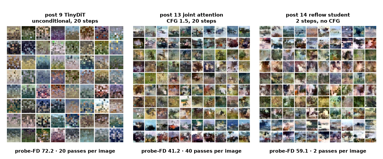
What you just built: A full scorecard of the series: probe-FD from 72.2 (post 9) to 41.2 (post 13 joint attention).
Where to Go Next
Everything in this series runs on pixels, at 32×32, on a CPU. Real 2026 image generators add three big things on top of what we built:
- Latent space. SD3 and FLUX don’t run the transformer on pixels. A separate autoencoder (a VAE) compresses a 1024×1024 image into a 128×128×16 “latent”, and the DiT does flow matching there. The DiT code doesn’t change, only
in_channelsandimg_size. - Text encoders. Instead of our 4 learned tokens per class, a frozen text encoder (CLIP, T5 or a small LLM) turns a prompt into a sequence of tokens that go into the MMDiT blocks from post 13.
- Distillation. Reflow is the first step. Methods like consistency models, progressive distillation and adversarial distillation get to 1 to 4 steps at high quality, and are how “turbo” and “schnell” models are made.
Note: We didn’t do latent space because training a good autoencoder is a project of its own (and a CPU won’t do it); with a pretrained VAE from the diffusers library you can swap it in.
Reading list
The papers behind every Expert post:
- Peebles and Xie, Scalable Diffusion Models with Transformers (DiT), ICCV 2023
- Lipman et al., Flow Matching for Generative Modeling, ICLR 2023
- Liu et al., Flow Straight and Fast: Learning to Generate and Transfer Data with Rectified Flow, ICLR 2023
- Esser et al., Scaling Rectified Flow Transformers for High-Resolution Image Synthesis (SD3), ICML 2024
- Ho and Salimans, Classifier-Free Diffusion Guidance, 2022
- Zhang and Sennrich, Root Mean Square Layer Normalization, NeurIPS 2019
- Shazeer, GLU Variants Improve Transformer, 2020
- Su et al., RoFormer: Enhanced Transformer with Rotary Position Embedding, 2021
- Dehghani et al., Scaling Vision Transformers to 22 Billion Parameters, ICML 2023
- Heo et al., Rotary Position Embedding for Vision Transformer, ECCV 2024
- Ho, Jain and Abbeel, Denoising Diffusion Probabilistic Models (DDPM), NeurIPS 2020
Recap
- Logit-normal timesteps put more training on the middle noise levels (SD3). On TinyDiT they made probe-FD worse (54.6 vs 50.3), so we don’t keep them at this scale.
- EMA weights are a free win: probe-FD 50.3 → 47.1 and class accuracy 32.7% → 36.2% at guidance 1.5, from the same training run.
- Reflow (rectified flow) fine-tunes a student on the teacher’s own noise-to-image pairs. One-step probe-FD went from 208.9 (teacher) to 61.3 (student), and 2-step from 93.0 to 59.1, with CFG baked in so each step is one forward pass.
- Across the series, probe-FD went from 72.2 (post 9) to 41.2 (post 13 joint attention), all trained on a CPU in minutes per run.
- Real 2026 models add latent space (a VAE), text encoders and stronger distillation on top of exactly these parts.
Next up: That’s the series: from a first tensor in post 1 to a class-conditional diffusion transformer with a 2026-style block, joint attention, guidance and few-step sampling, all in code you’ve run yourself. Go back to the PyTorch Tutorial 2026: From Tensors to Tiny Diffusion hub for the full list, and try the GPU settings if you have one: the same code, bigger and longer, makes noticeably better pictures.
Series: PyTorch Tutorial 2026 (14 posts)
- Post 1: PyTorch Tutorial 2026: From Tensors to Tiny Diffusion
- Post 2: PyTorch Tensors Explained: Shapes, Broadcasting, and Images as Arrays
- Post 3: PyTorch Autograd: How backward() Builds Gradients
- Post 4: PyTorch DataLoader Explained: Datasets, Batches, and Image Folders
- Post 5: PyTorch nn.Module and the Training Loop: Layers, Loss, and Checkpoints
- Post 6: Attention and the Transformer Block in PyTorch
- Post 7: Patch Embeddings in PyTorch: How a Transformer Reads an Image
- Post 8: Flow Matching in PyTorch: Train a Model to Follow a Straight Line
- Post 9: Build a Tiny Diffusion Transformer in PyTorch (DiT from Scratch)
- Post 10: torch.compile, Mixed Precision, and SDPA: Speed Up TinyDiT
- Post 11: RMSNorm, QK-Norm, SwiGLU, and 2D RoPE in a Tiny DiT
- Post 12: adaLN-Zero and Classifier-Free Guidance in PyTorch
- Post 13: MMDiT Joint Attention in PyTorch: Two Streams, One Generator
- Post 14: Train and Sample Like 2026: Logit-Normal Steps, EMA, and Few-Step Flow (you are here)
← Previous: Post 13: MMDiT Joint Attention in PyTorch: Two Streams, One Generator
Back to the start: Post 1: PyTorch Tutorial 2026: From Tensors to Tiny Diffusion