PyTorch nn.Module and the Training Loop: Layers, Loss, and Checkpoints
Where you are: Post 5 of 14 in PyTorch Tutorial 2026 · about 12 min read
What you’ll build: nn.Module models, the ResidualFFN block (the feed-forward half of every TinyDiT block), AdamW, and tinydit/trainer.py, a reusable training loop with evaluation and resumable checkpoints, proven on real CIFAR-10 data.
You’ll need: Post 3 (autograd and the training heartbeat) and Post 4 (the CIFAR-10 loaders).
In this post:
- Introduction
- Step 1/6: nn.Module: The Shape of Every Model
- Step 2/6: The Pieces of a Transformer Feed-Forward Block
- Step 3/6: The ResidualFFN Module
- Step 4/6: AdamW: The Optimizer
- Step 5/6: The PyTorch Training Loop and the Trainer
- Step 6/6: Prove It: Clean Up Noisy Image Patches
- Recap
Series: PyTorch Tutorial 2026 (14 posts)
- Post 1: PyTorch Tutorial 2026: From Tensors to Tiny Diffusion
- Post 2: PyTorch Tensors Explained: Shapes, Broadcasting, and Images as Arrays
- Post 3: PyTorch Autograd: How backward() Builds Gradients
- Post 4: PyTorch DataLoader Explained: Datasets, Batches, and Image Folders
- Post 5: PyTorch nn.Module and the Training Loop: Layers, Loss, and Checkpoints (you are here)
- Post 6: Attention and the Transformer Block in PyTorch
- Post 7: Patch Embeddings in PyTorch: How a Transformer Reads an Image
- Post 8: Flow Matching in PyTorch: Train a Model to Follow a Straight Line
- Post 9: Build a Tiny Diffusion Transformer in PyTorch (DiT from Scratch)
- Post 10: torch.compile, Mixed Precision, and SDPA: Speed Up TinyDiT
- Post 11: RMSNorm, QK-Norm, SwiGLU, and 2D RoPE in a Tiny DiT
- Post 12: adaLN-Zero and Classifier-Free Guidance in PyTorch
- Post 13: MMDiT Joint Attention in PyTorch: Two Streams, One Generator
- Post 14: Train and Sample Like 2026: Logit-Normal Steps, EMA, and Few-Step Flow
Introduction
Every model you will ever train in PyTorch runs the same six-line heartbeat: zero the gradients, run the forward pass, compute the loss, call backward, take an optimizer step, repeat. This post turns that PyTorch training loop into a reusable Trainer with checkpoints, and introduces nn.Module, the class every layer and model in PyTorch is built on.
Along the way we build the pieces a transformer is made of (nn.Linear, GELU, LayerNorm and the residual connection) and combine them into a ResidualFFN, the feed-forward half of every TinyDiT block. Then we prove the whole thing on real CIFAR-10 data.
In PyTorch Autograd: How backward() Builds Gradients we fit a line with raw tensors and a hand-written update. In PyTorch DataLoader Explained: Datasets, Batches, and Image Folders we built loaders that hand us (images, labels) batches. Now we replace the raw tensors with modules and the hand-written update with AdamW; this is the last foundation post before we start building the generator.
Step 1/6: nn.Module: The Shape of Every Model
In this step: We write our first nn.Module and see how it registers layers and parameters for the optimizer.
An nn.Module is a Python class that does two jobs:
- holds parameters: any layer you assign as an attribute in
__init__is registered, along with its weights; - defines
forward: the computation from input to output.
import torch
from torch import nn

class TwoLayer(nn.Module):
    def __init__(self, d_in: int, d_hidden: int, d_out: int):
        super().__init__()                      # always call this first
        self.fc1 = nn.Linear(d_in, d_hidden)    # assigning a layer registers it
        self.act = nn.GELU()
        self.fc2 = nn.Linear(d_hidden, d_out)

    def forward(self, x: torch.Tensor) -> torch.Tensor:
        return self.fc2(self.act(self.fc1(x)))

torch.manual_seed(0)
model = TwoLayer(48, 64, 48)
print(model)
for name, p in model.named_parameters():
    print(f"{name:10s} {str(tuple(p.shape)):10s} requires_grad={p.requires_grad}")
print("total params:", sum(p.numel() for p in model.parameters()))
print("output:", tuple(model(torch.randn(5, 48)).shape)) # call the module, not .forward()TwoLayer(
(fc1): Linear(in_features=48, out_features=64, bias=True)
(act): GELU(approximate='none')
(fc2): Linear(in_features=64, out_features=48, bias=True)
)
fc1.weight (64, 48) requires_grad=True
fc1.bias (64,) requires_grad=True
fc2.weight (48, 64) requires_grad=True
fc2.bias (48,) requires_grad=True
total params: 6256
output: (5, 48)Some things to notice:
model.parameters()andnamed_parameters()find every weight automatically, including weights inside sub-modules. This is the list the optimizer will update.- Every weight has
requires_grad=True, so autograd (PyTorch Autograd: How backward() Builds Gradients) tracks it with no extra work from you. - You call
model(x), notmodel.forward(x). Calling the module runsforwardplus PyTorch’s hooks. - Modules nest. A transformer is a module made of blocks, which are modules made of Linears and LayerNorms.
print(model)shows the tree.
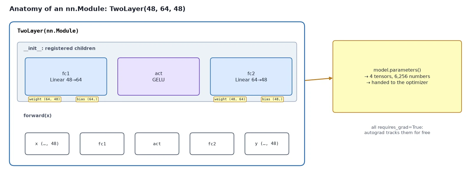
What you just built: A two-layer nn.Module whose parameters PyTorch finds and tracks automatically.
Step 2/6: The Pieces of a Transformer Feed-Forward Block
In this step: We meet the four pieces a transformer’s feed-forward network is made of: nn.Linear, GELU, LayerNorm and the residual connection.
The feed-forward network (FFN) in a transformer is simple: normalize, a Linear that widens each token, a nonlinearity, a Linear that narrows it back, and a residual add. All four pieces are introduced here because the transformer reuses every one of them.
nn.Linear
\underbrace{y}_{(\dots,\ d_{\text{out}})} = \underbrace{x}_{(\dots,\ d_{\text{in}})}\, \underbrace{W^{\top}}_{(d_{\text{in}},\ d_{\text{out}})} + \underbrace{b}_{(d_{\text{out}})}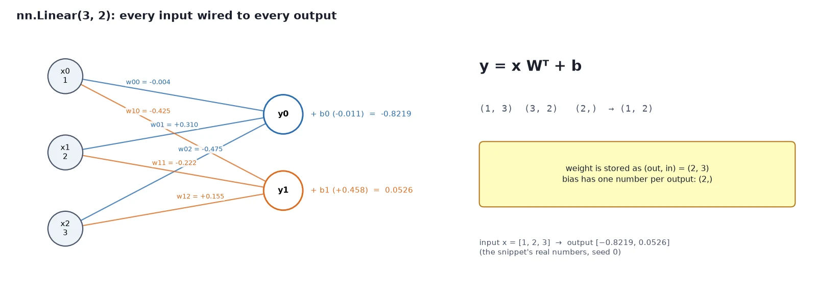
import torch
from torch import nn

torch.manual_seed(0)
lin = nn.Linear(3, 2)                 # weight (2, 3), bias (2,)
x = torch.tensor([[1.0, 2.0, 3.0]])   # one input vector, as a batch of 1

by_hand = x @ lin.weight.T + lin.bias
print(lin(x))
print(by_hand)
print("weight is a Parameter:", isinstance(lin.weight, nn.Parameter))

tokens = torch.randn(4, 64, 3)        # extra leading axes are fine: applied to every token
print(tuple(lin(tokens).shape))tensor([[-0.8219, 0.0526]], grad_fn=<AddmmBackward0>)
tensor([[-0.8219, 0.0526]], grad_fn=<AddBackward0>)
weight is a Parameter: True
(4, 64, 2)nn.Linear acts on the last axis only, so the same layer works on one vector (3,), a batch (N, 3), or a batch of token sequences (N, L, 3). That last case is how a transformer applies one FFN to every token at once.
What it is: a learned map from one vector to another.
Why it works: almost every learned transform in a transformer is a Linear: Q, K, V, the attention output, both halves of the FFN, the patch embedding.
How it works: y = xW^\top + b on the last axis. weight and bias are nn.Parameters.
GELU
\begin{aligned} \operatorname{GELU}(x) &= x \cdot \underbrace{\Phi(x)}_{\text{chance a standard normal is} \,\le\, x} \\ &\approx \tfrac{1}{2}\,x\left(1 + \tanh\!\Big[\sqrt{2/\pi}\,\big(x + 0.044715\,x^{3}\big)\Big]\right) \end{aligned}import math
import torch
from torch import nn
x = torch.tensor([-3.0, -1.0, -0.5, 0.0, 0.5, 1.0, 3.0])
exact = nn.GELU()(x) # x * Phi(x)
tanh = nn.GELU(approximate="tanh")(x) # the fast form DiT and FLUX use
by_hand = x * 0.5 * (1 + torch.erf(x / math.sqrt(2)))
torch.set_printoptions(precision=4)
print("GELU :", exact)
print("by hand :", by_hand)
print("tanh form :", tanh)
print("ReLU :", torch.relu(x))
# Without a nonlinearity, two Linears collapse into one:
torch.manual_seed(0)
a, b = nn.Linear(4, 8), nn.Linear(8, 4)
v = torch.randn(3, 4)
W = b.weight @ a.weight
c = b.weight @ a.bias + b.bias
print("Linear(Linear(x)) is one Linear:", torch.allclose(b(a(v)), v @ W.T + c, atol=1e-6))GELU : tensor([-0.0041, -0.1587, -0.1543, 0.0000, 0.3457, 0.8413, 2.9959])
by hand : tensor([-0.0040, -0.1587, -0.1543, 0.0000, 0.3457, 0.8413, 2.9960])
tanh form : tensor([-0.0036, -0.1588, -0.1543, 0.0000, 0.3457, 0.8412, 2.9964])
ReLU : tensor([0.0000, 0.0000, 0.0000, 0.0000, 0.5000, 1.0000, 3.0000])
Linear(Linear(x)) is one Linear: True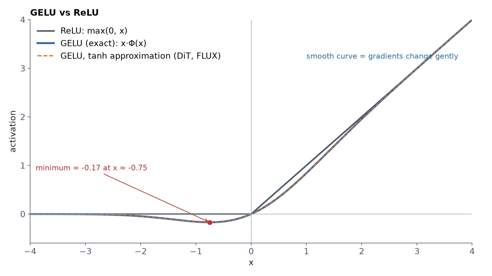
The last line of that output is the reason nonlinearities exist: two Linears in a row are just one Linear, no matter how wide. GELU breaks that, so stacked layers can learn curved, complicated functions.
What it is: a smooth nonlinearity between Linears.
Why it works: Linears stacked without a nonlinearity collapse into one Linear. GELU’s smooth curve keeps gradients well-behaved; it is the default in the original DiT MLP and in FLUX.1’s feed-forward.
How it works: x\,\Phi(x), or the tanh approximation. nn.GELU(approximate="tanh").
LayerNorm
\operatorname{LN}(x) = \underbrace{\gamma}_{\text{learned scale}} \odot \frac{x - \overbrace{\mu}^{\text{mean of this token's } D \text{ features}}}{\sqrt{\underbrace{\sigma^{2}}_{\text{their variance}} + \epsilon}} + \underbrace{\beta}_{\text{learned shift}}import torch
from torch import nn
torch.manual_seed(0)
x = torch.randn(2, 64, 256) * 5 + 3 # tokens with a big scale and offset
ln = nn.LayerNorm(256)
y = ln(x)
mean = x.mean(dim=-1, keepdim=True) # per token, over its 256 features
var = x.var(dim=-1, keepdim=True, unbiased=False)
by_hand = (x - mean) / torch.sqrt(var + ln.eps) * ln.weight + ln.bias
print("matches by-hand formula:", torch.allclose(y, by_hand, atol=1e-5))
print("before: mean %.2f std %.2f" % (x[0, 0].mean(), x[0, 0].std()))
print("after : mean %.2f std %.2f" % (y[0, 0].mean().item(), y[0, 0].std().item()))
print("learnable gamma, beta:", tuple(ln.weight.shape), tuple(ln.bias.shape))matches by-hand formula: True
before: mean 3.13 std 4.70
after : mean -0.00 std 1.00
learnable gamma, beta: (256,) (256,)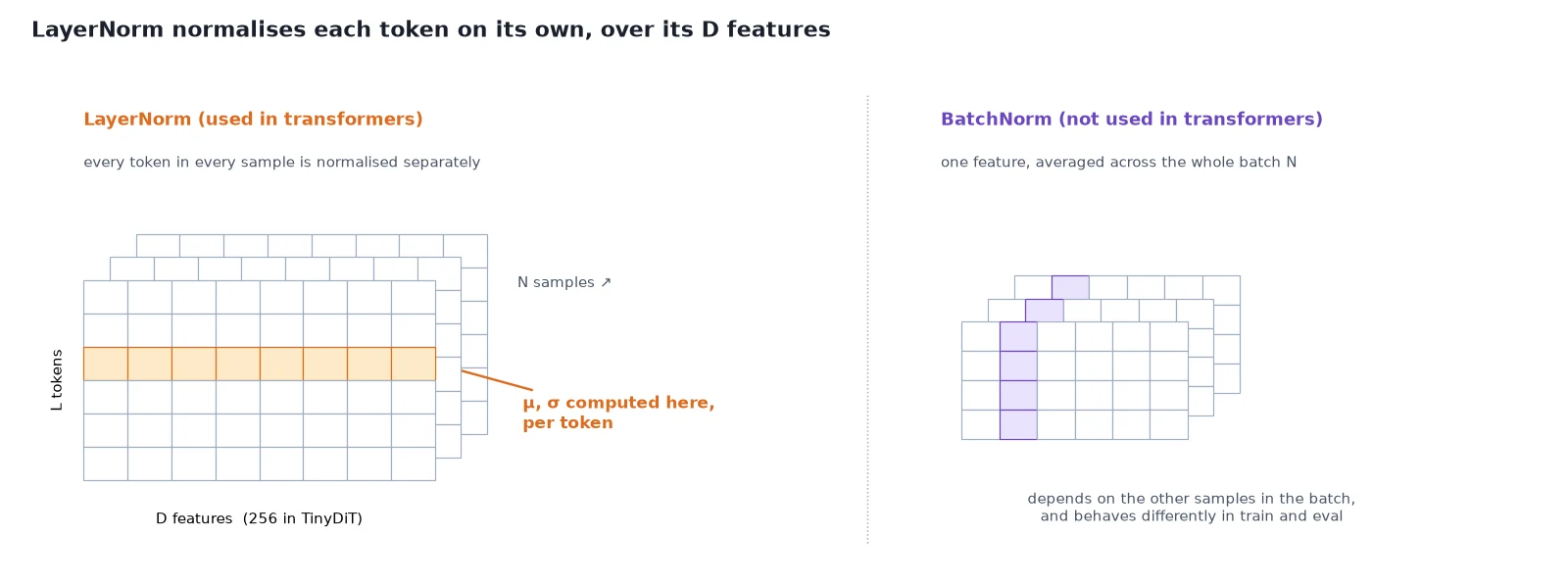
What it is: a layer that keeps each token’s features on a stable scale.
Why it works: deep stacks drift: values grow or shrink layer after layer. Normalizing each token to mean 0, std 1 (then learning a scale and shift) makes training far less brittle.
How it works: mean and variance over the last axis (D), per token, then \gamma and \beta. nn.LayerNorm(D).
The residual connection
\underbrace{y}_{\text{output}} = \underbrace{x}_{\text{skip: passes straight through}} + \underbrace{F(x)}_{\text{the block's correction}}What it is: a skip path that lets a block adjust its input instead of replacing it.
Why it works: the block only has to learn a correction, and gradients can skip straight past it, so deep stacks still train. Step 3 measures this: 16 blocks reach loss 0.065 with skips vs 0.143 without.
How it works: out = x + block(x). Shapes must match.
What you just built: The four building blocks of a transformer FFN: nn.Linear, GELU, LayerNorm and the residual add, each tested on its own.
Step 3/6: The ResidualFFN Module
In this step: We combine the four pieces into ResidualFFN, the feed-forward half of every TinyDiT block, and measure why the residual matters.
Put the pieces together and you get the feed-forward half of a transformer block. We split it into two classes in tinydit/layers.py.
FeedForward is the bare Linear → GELU → Linear. Later posts reuse it inside other block designs:
"""Feed-forward pieces (post 5). TransformerBlock (post 6) and DiT blocks (post 9+) reuse FeedForward."""
import torch
from torch import nn


class FeedForward(nn.Module):
    """Linear -> GELU -> Linear. (N, L, dim) -> (N, L, dim). No norm, no residual."""

    def __init__(self, dim: int, mlp_ratio: float = 4.0, dropout: float = 0.0):
        super().__init__()
        hidden = int(dim * mlp_ratio)
        self.fc1 = nn.Linear(dim, hidden)
        self.act = nn.GELU(approximate="tanh")
        self.fc2 = nn.Linear(hidden, dim)
        self.drop = nn.Dropout(dropout)

    def forward(self, x: torch.Tensor) -> torch.Tensor:
return self.drop(self.fc2(self.act(self.fc1(x))))ResidualFFN wraps it with a pre-norm LayerNorm and the residual add:
class ResidualFFN(nn.Module):
    """Pre-norm residual feed-forward: x + FeedForward(LayerNorm(x)). Shape in == shape out."""

    def __init__(self, dim: int, mlp_ratio: float = 4.0, dropout: float = 0.0):
        super().__init__()
        self.norm = nn.LayerNorm(dim)
        self.mlp = FeedForward(dim, mlp_ratio, dropout)

    def forward(self, x: torch.Tensor) -> torch.Tensor:
        return x + self.mlp(self.norm(x))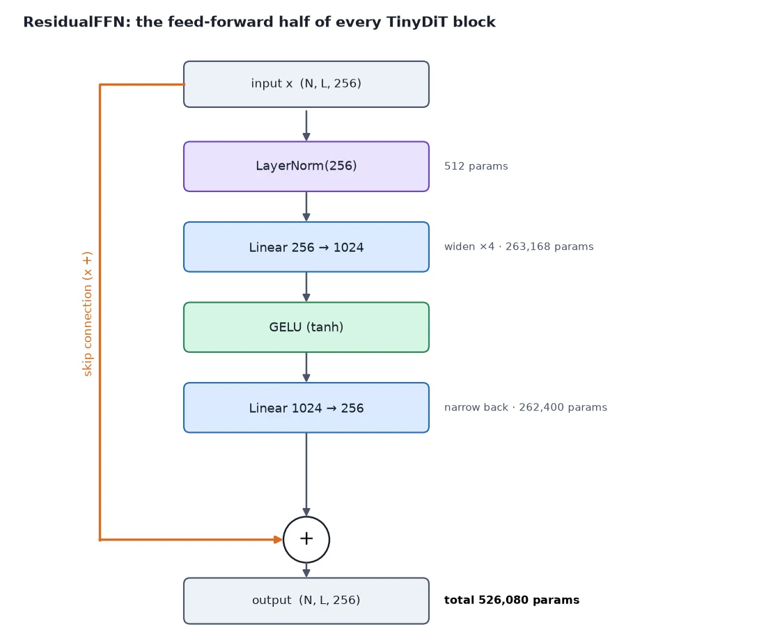
We use the tanh form of GELU (approximate="tanh") because that’s what the original DiT MLP uses, and FLUX.1’s feed-forward too. The hidden layer is 4× wider than the token (mlp_ratio=4.0), the standard transformer choice.
First, build one block and count its parameters:
import torch
from torch import nn
from tinydit.layers import ResidualFFN

torch.manual_seed(0)
block = ResidualFFN(dim=256)
print(block)
x = torch.randn(2, 64, 256)
print(tuple(block(x).shape), "| params:", sum(p.numel() for p in block.parameters()))Then train the same deep stack of 16 blocks twice, with and without the x +:
# Why residuals help: train the same deep stack of 16 blocks, with and without "x +".
class NoSkip(nn.Module):
    def __init__(self, blk):
        super().__init__(); self.blk = blk
    def forward(self, h):
        return self.blk.mlp(self.blk.norm(h))      # same layers, residual removed

def train_stack(residual: bool, depth: int = 16, steps: int = 300) -> float:
    torch.manual_seed(0)
    teacher = nn.Linear(32, 32)                     # a random target function to imitate
    blocks = [ResidualFFN(32) for _ in range(depth)]
    model = nn.Sequential(*(blocks if residual else [NoSkip(b) for b in blocks]))
    opt = torch.optim.AdamW(model.parameters(), lr=1e-3)
    for _ in range(steps):
        inp = torch.randn(128, 32)
        with torch.no_grad():
            target = torch.tanh(teacher(inp))
        loss = ((model(inp) - target) ** 2).mean()
        opt.zero_grad(); loss.backward(); opt.step()
    return loss.item()

print(f"16 blocks WITH residual    -> final loss {train_stack(True):.4f}")
print(f"16 blocks WITHOUT residual -> final loss {train_stack(False):.4f}")ResidualFFN(
(norm): LayerNorm((256,), eps=1e-05, elementwise_affine=True, bias=True)
(mlp): FeedForward(
(fc1): Linear(in_features=256, out_features=1024, bias=True)
(act): GELU(approximate='tanh')
(fc2): Linear(in_features=1024, out_features=256, bias=True)
(drop): Dropout(p=0.0, inplace=False)
)
)
(2, 64, 256) | params: 526080
16 blocks WITH residual -> final loss 0.0647
16 blocks WITHOUT residual -> final loss 0.1432The second half of that output shows why the residual matters. The same 16 blocks, trained the same way, reach a clearly lower loss when each block adds to its input instead of replacing it.
Why it works: Every block can start out as “almost nothing changes” and learn small corrections, and the gradient has a direct path back through the x + to the early blocks.
ResidualFFN: what, why, how
What it is: the “each token thinks on its own” half of a transformer block. It transforms every token’s features independently.
Why it works: widening to 4D gives the GELU lots of room to carve out useful features before the second Linear compresses them back. Pre-norm keeps the input scale steady, and the residual keeps the block easy to train when you stack many of them.
How it works: x + fc2(gelu(fc1(layernorm(x)))), with fc1: D → 4D and fc2: 4D → D. At D = 256, that’s 526,080 parameters per block.
What you just built: FeedForward and ResidualFFN in tinydit/layers.py: 526,080 parameters per block at D = 256, shape in equals shape out.
Step 4/6: AdamW: The Optimizer
In this step: We replace the hand-written update from post 3 with AdamW, and check PyTorch’s update against the formula.
In post 3 we updated weights by hand: w -= lr * w.grad. That is plain SGD (stochastic gradient descent). It uses one learning rate for every weight, which works badly when some weights get huge gradients and others tiny ones.
Adam keeps two running averages for every weight: the average gradient (momentum, so steps don’t zig-zag) and the average squared gradient (so each weight’s step is scaled by its own typical gradient size).
AdamW (Loshchilov and Hutter, 2019) adds weight decay the right way: as a separate small pull toward zero, instead of mixing it into the gradient where Adam’s scaling would distort it. Transformers, from LLMs to DiT and SD3, are trained with AdamW, and so is TinyDiT.
\begin{aligned} m_t &= \beta_1 m_{t-1} + (1-\beta_1)\,g_t && \text{mean of gradients (momentum)}\\ v_t &= \beta_2 v_{t-1} + (1-\beta_2)\,g_t^{2} && \text{mean of squared gradients}\\ \hat m_t &= \tfrac{m_t}{1-\beta_1^{t}},\quad \hat v_t = \tfrac{v_t}{1-\beta_2^{t}} && \text{bias correction}\\ w_t &= w_{t-1} - \eta\,\lambda\, w_{t-1} && \text{decoupled weight decay}\\ &\quad - \eta\,\frac{\hat m_t}{\sqrt{\hat v_t} + \epsilon} && \text{then the Adam step} \end{aligned}To be sure that’s really what PyTorch does, here is one parameter updated by torch.optim.AdamW and by those four lines, side by side:
import torch

torch.manual_seed(0)
w = torch.randn(5, requires_grad=True)
w_ref = w.detach().clone()
opt = torch.optim.AdamW([w], lr=1e-2, betas=(0.9, 0.999), eps=1e-8, weight_decay=0.1)

m = torch.zeros(5); v = torch.zeros(5)
for t in range(1, 4):
    loss = (w ** 2).sum()
    opt.zero_grad(); loss.backward()
    g = w.grad.detach().clone()
    opt.step()

    # The same update by hand:
    w_ref *= 1 - 1e-2 * 0.1                       # decoupled weight decay
    m = 0.9 * m + 0.1 * g                         # 1st moment: running mean of gradients
    v = 0.999 * v + 0.001 * g * g                 # 2nd moment: running mean of squared gradients
    m_hat, v_hat = m / (1 - 0.9 ** t), v / (1 - 0.999 ** t)   # bias correction
    w_ref -= 1e-2 * m_hat / (v_hat.sqrt() + 1e-8)
print(f"step {t}: torch == by hand? {torch.allclose(w.detach(), w_ref, atol=1e-6)}")step 1: torch == by hand? True
step 2: torch == by hand? True
step 3: torch == by hand? TrueIn practice you never write this by hand. You hand the optimizer model.parameters() and call optimizer.step().
What it is: the optimizer that updates weights from gradients.
Why it works: momentum smooths noisy gradients; per-weight scaling by \sqrt{\hat v} gives every weight a sensible step size; decoupled weight decay regularizes without being distorted by that scaling.
How it works: the four-line update above. torch.optim.AdamW(model.parameters(), lr=...).
What you just built: A verified understanding of AdamW: PyTorch’s update matches the formula step by step.
Step 5/6: The PyTorch Training Loop and the Trainer
In this step: We package the training heartbeat into tinydit/trainer.py, with train/eval modes, gradient clipping and checkpoints.
Here is the heartbeat, now with real PyTorch objects instead of hand-written updates:
\begin{aligned} &\underbrace{\texttt{zero\_grad()}}_{\text{clear old grads}} \rightarrow \underbrace{\texttt{model(x)}}_{\text{forward}} \rightarrow \underbrace{\texttt{loss\_fn(...)}}_{\text{how wrong?}} \\ &\rightarrow \underbrace{\texttt{loss.backward()}}_{\text{fill .grad}} \rightarrow \underbrace{\texttt{optimizer.step()}}_{\text{AdamW update}} \rightarrow \text{repeat} \end{aligned}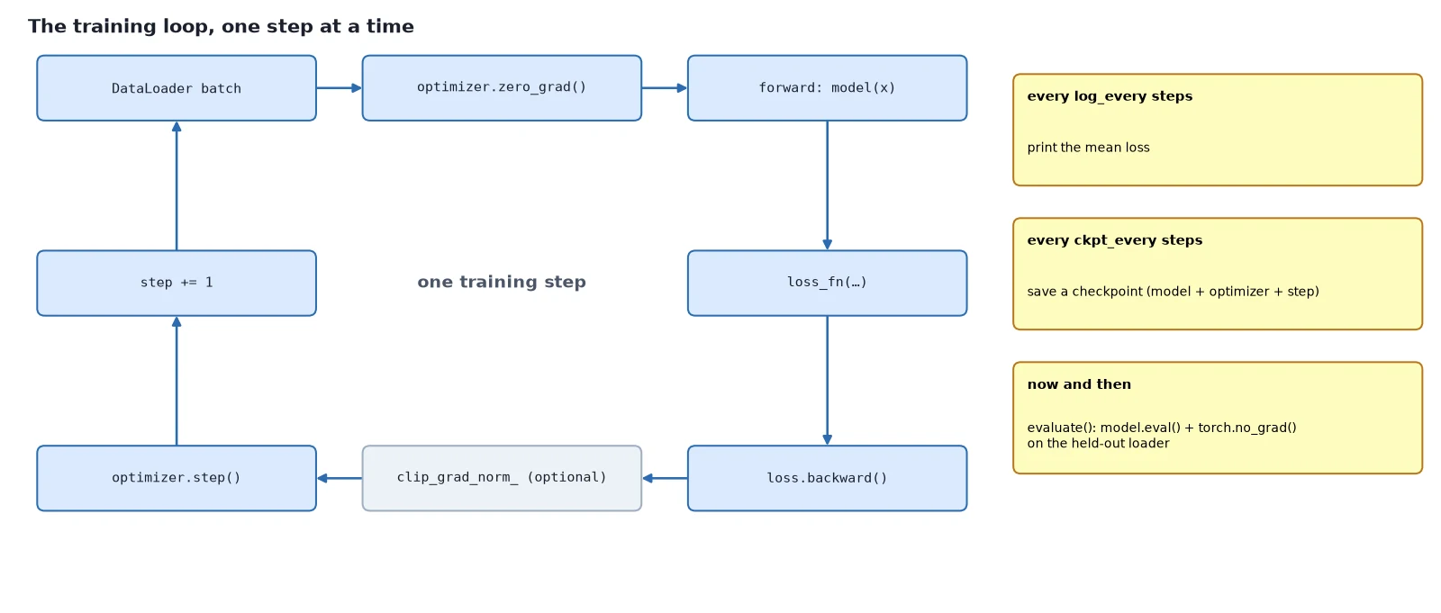
model.train() and model.eval()
Some layers behave differently while training. Dropout randomly zeroes features during training and does nothing at evaluation. The module’s training flag controls this:
import torch
from torch import nn

torch.manual_seed(0)
model = nn.Sequential(nn.Linear(8, 8), nn.Dropout(p=0.5))
x = torch.ones(1, 8)

model.train()                          # dropout active: random zeros, survivors scaled x2
print("train:", torch.equal(model(x), model(x)))
model.eval()                           # dropout off: deterministic
with torch.no_grad():                  # and no graph, for evaluation
    print("eval :", torch.equal(model(x), model(x)))
print("model.training =", model.training)train: False
eval : True
model.training = FalseNote: Rule of thumb: call model.train() before training steps and model.eval() plus torch.no_grad() for evaluation and sampling. TinyDiT has no dropout by default, but the habit protects you when you add layers that care.
The Trainer, piece by piece
tinydit/trainer.py packages the loop so every later post can reuse it. The key design choice is the loss function signature, loss_fn(model, batch) -> loss. The Trainer doesn’t know or care what the task is; in post 8 the flow-matching loss plugs in here, and the Trainer doesn’t change.
The file opens with that signature and a helper that moves any batch (a tensor, tuple, list or dict) to the device:
"""A small, reusable training loop with checkpoints (post 5).

A loss function has the signature   loss_fn(model, batch) -> scalar tensor.
`batch` is whatever the DataLoader yields (for our loaders: (images, labels)).
Flow matching (post 8) plugs in here without changing the Trainer.
"""
from pathlib import Path
from typing import Callable, Iterable

import torch
from torch import nn

LossFn = Callable[[nn.Module, object], torch.Tensor]


def move_to(batch, device):
    """Move a tensor, or a tuple/list/dict of tensors, to `device`."""
    if torch.is_tensor(batch):
        return batch.to(device, non_blocking=True)
    if isinstance(batch, (list, tuple)):
        return type(batch)(move_to(b, device) for b in batch)
    if isinstance(batch, dict):
        return {k: move_to(v, device) for k, v in batch.items()}
return batchThe constructor moves the model to the device and creates AdamW if you don’t pass an optimizer:
class Trainer:
    def __init__(self, model: nn.Module, loss_fn: LossFn,
                 optimizer: torch.optim.Optimizer | None = None,
                 device: str | torch.device = "cpu",
                 lr: float = 3e-4, weight_decay: float = 0.0,
                 max_grad_norm: float | None = 1.0):
        self.device = torch.device(device)
        self.model = model.to(self.device)
        self.loss_fn = loss_fn
        self.optimizer = optimizer or torch.optim.AdamW(
            self.model.parameters(), lr=lr, weight_decay=weight_decay)
        self.max_grad_norm = max_grad_norm
self.step = 0 # optimizer steps taken so fartrain_step is the heartbeat itself, with gradient clipping before the optimizer step:
    def train_step(self, batch) -> float:
        """One heartbeat: zero_grad, forward + loss, backward, (clip), step."""
        self.model.train()
        batch = move_to(batch, self.device)
        self.optimizer.zero_grad(set_to_none=True)
        loss = self.loss_fn(self.model, batch)
        loss.backward()
        if self.max_grad_norm is not None:
            nn.utils.clip_grad_norm_(self.model.parameters(), self.max_grad_norm)
        self.optimizer.step()
        self.step += 1
return loss.item()fit repeats train_step over the loader until max_steps, logging and saving checkpoints on the way:
    def fit(self, loader: Iterable, max_steps: int, log_every: int = 100,
            ckpt_path: str | Path | None = None, ckpt_every: int | None = None) -> list[float]:
        """Loop over `loader` (re-iterating as needed) until self.step == max_steps."""
        losses: list[float] = []
        while self.step < max_steps:
            for batch in loader:
                losses.append(self.train_step(batch))
                if log_every and self.step % log_every == 0:
                    recent = losses[-log_every:]
                    print(f"step {self.step:6d} | loss {sum(recent) / len(recent):.4f}")
                if ckpt_path and ckpt_every and self.step % ckpt_every == 0:
                    self.save(ckpt_path)
                if self.step >= max_steps:
                    break
        if ckpt_path:
            self.save(ckpt_path)
return lossesevaluate averages the loss over a held-out loader, without gradients:
    @torch.no_grad()
    def evaluate(self, loader: Iterable, max_batches: int | None = None) -> float:
        """Average loss over a held-out loader, in eval mode, without gradients."""
        self.model.eval()
        total, count = 0.0, 0
        for i, batch in enumerate(loader):
            if max_batches is not None and i >= max_batches:
                break
            batch = move_to(batch, self.device)
            total += self.loss_fn(self.model, batch).item()
            count += 1
        self.model.train()
return total / max(count, 1)save and load store and restore the model, the optimizer state and the step count:
    def save(self, path: str | Path, **extra) -> None:
        path = Path(path)
        path.parent.mkdir(parents=True, exist_ok=True)
        torch.save({"model": self.model.state_dict(),
                    "optimizer": self.optimizer.state_dict(),
                    "step": self.step,
                    **extra}, path)

    def load(self, path: str | Path) -> dict:
        ckpt = torch.load(path, map_location=self.device, weights_only=True)
        self.model.load_state_dict(ckpt["model"])
        self.optimizer.load_state_dict(ckpt["optimizer"])
        self.step = ckpt["step"]
return ckptA few details worth calling out:
zero_grad(set_to_none=True)sets gradients toNoneinstead of filling them with zeros. That’s slightly faster, and it’s the default in PyTorch 2.x.clip_grad_norm_caps the total gradient size at 1.0. One unlucky batch can produce a huge gradient, and clipping keeps it from throwing the weights far off course. Transformer trainers almost always do this.evaluateuses@torch.no_grad()andmodel.eval(), then switches back to train mode.
Why it works: save stores the model, the optimizer state and the step count. The optimizer state matters: AdamW’s running averages m and v are part of training, and without them a resumed run takes a few clumsy steps.
What you just built: tinydit/trainer.py: a Trainer with train_step, fit, evaluate, save and load that accepts any loss_fn(model, batch).
Step 6/6: Prove It: Clean Up Noisy Image Patches
In this step: We train a small patch denoiser on real CIFAR-10 data with the Trainer, then resume it from a checkpoint.
Let’s train something real. The task is a first taste of diffusion: cut CIFAR-10 images into 4×4 patches (48 numbers each, using patchify, which post 7 explains in detail), add Gaussian noise, and train a model to recover the clean patch.
The model is a Linear in, two ResidualFFN blocks, and a Linear out. It lives in examples/patch_denoiser.py:
"""A small model that cleans up noisy 4x4 image patches (post 5).

It proves the Trainer works on real CIFAR-10 data, and it is a first taste of the
"predict something clean from something noisy" idea behind diffusion.
"""
import torch
import torch.nn.functional as F
from torch import nn

from tinydit.layers import ResidualFFN
from tinydit.patches import patchify

NOISE = 0.5  # standard deviation of the Gaussian noise we add


class PatchDenoiser(nn.Module):
    """noisy patch (48 numbers) -> clean patch (48 numbers), applied to every patch."""

    def __init__(self, patch_dim: int = 48, dim: int = 128, depth: int = 2):
        super().__init__()
        self.inp = nn.Linear(patch_dim, dim)
        self.blocks = nn.Sequential(*[ResidualFFN(dim) for _ in range(depth)])
        self.norm = nn.LayerNorm(dim)
        self.out = nn.Linear(dim, patch_dim)

    def forward(self, x: torch.Tensor) -> torch.Tensor:
return self.out(self.norm(self.blocks(self.inp(x))))The loss adds noise to the clean patches and asks the model to recover them:
def denoise_loss(model: nn.Module, batch) -> torch.Tensor:
    images, _labels = batch                     # (N, 3, 32, 32) in [-1, 1]
    clean = patchify(images, 4)                 # (N, 64, 48): 64 patches of 4x4x3
    noisy = clean + NOISE * torch.randn_like(clean)
return F.mse_loss(model(noisy), clean)In math, it is the mean squared error between the prediction and the clean patch:
\begin{gathered} \mathcal{L} = \frac{1}{N}\sum \big\| f_\theta(\underbrace{x + 0.5\,\varepsilon}_{\text{noisy patch}}) - \underbrace{x}_{\text{clean patch}} \big\|^2 \\ \varepsilon \sim \mathcal{N}(0, I) \end{gathered}Train for 300 steps on 8,192 images (CPU-friendly), measuring loss on held-out test images before and after:
import torch
from tinydit import get_device
from tinydit.data import get_cifar10, make_loader
from tinydit.trainer import Trainer
from examples.patch_denoiser import PatchDenoiser, denoise_loss, NOISE

torch.manual_seed(0)
train_loader = make_loader(get_cifar10("data", train=True, limit=8192), batch_size=128, num_workers=2)
test_loader = make_loader(get_cifar10("data", train=False, limit=1024), batch_size=256,
                          shuffle=False, num_workers=0)

model = PatchDenoiser()
print("params:", sum(p.numel() for p in model.parameters()))
trainer = Trainer(model, denoise_loss, device=get_device(), lr=1e-3)

print("held-out loss before:", round(trainer.evaluate(test_loader), 4))
trainer.fit(train_loader, max_steps=300, log_every=50, ckpt_path="checkpoints/denoiser.pt")
print("held-out loss after: ", round(trainer.evaluate(test_loader), 4))
print("baseline (return the noisy patch unchanged):", NOISE ** 2)params: 276656
held-out loss before: 0.6019
step 50 | loss 0.0737
step 100 | loss 0.0333
step 150 | loss 0.0320
step 200 | loss 0.0313
step 250 | loss 0.0308
step 300 | loss 0.0304
held-out loss after: 0.0301
baseline (return the noisy patch unchanged): 0.25Read the numbers from top to bottom:
- Before training, the random model scores 0.60, worse than doing nothing at all.
- A model that just returns the noisy patch unchanged would score 0.5^2 = 0.25, because that’s exactly the noise we added.
- After 300 steps (about half a minute on a laptop CPU), the held-out error is 0.030, about 8× lower than doing nothing. The model has learned what real image patches look like well enough to strip most of the noise off them.
- The held-out loss (0.0301) matches the training loss (0.0304), so the model isn’t just memorizing the training images.
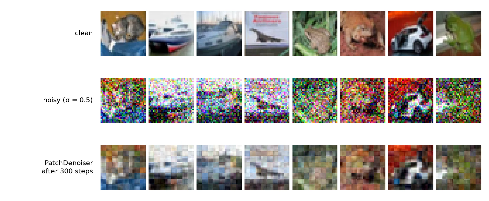
Note: This model cleans each patch in isolation. It can’t use the sky in the next patch to decide what this patch should look like. Letting patches talk to each other is the job of attention, and that’s next.
Resume from a checkpoint
Training on Colab can be interrupted at any time. The checkpoint lets us pick up exactly where we stopped:
import torch
from tinydit import get_device
from tinydit.data import get_cifar10, make_loader
from tinydit.trainer import Trainer
from examples.patch_denoiser import PatchDenoiser, denoise_loss

trainer = Trainer(PatchDenoiser(), denoise_loss, device=get_device(), lr=1e-3)
ckpt = trainer.load("checkpoints/denoiser.pt")        # model + optimizer + step
print("resumed at step", trainer.step, "| checkpoint keys:", sorted(ckpt))

loader = make_loader(get_cifar10("data", train=True, limit=8192), batch_size=128, num_workers=2)
trainer.fit(loader, max_steps=400, log_every=50, ckpt_path="checkpoints/denoiser.pt")
print("now at step", trainer.step)resumed at step 300 | checkpoint keys: ['model', 'optimizer', 'step']
step 350 | loss 0.0300
step 400 | loss 0.0298
now at step 400The step counter, the weights and AdamW’s running averages all came back, and training continued from step 300 to 400. TinyDiT runs take hours instead of seconds, so you’ll be glad of this in post 9.
What you just built: A PatchDenoiser trained with the Trainer that cuts the held-out error from 0.25 (do nothing) to 0.030, and resumes cleanly from its checkpoint.
Recap
nn.Moduleregisters layers and parameters in__init__and definesforward.model.parameters()is what the optimizer updates.- The transformer FFN is LayerNorm → Linear (×4 wider) → GELU → Linear → residual add. In TinyDiT it’s
ResidualFFN. - AdamW is Adam with decoupled weight decay. We checked PyTorch’s update against the formula, step by step.
- The PyTorch training loop is zero_grad → forward → loss → backward → (clip) → step. The
Trainerpackages it with evaluation and resumable checkpoints, and accepts anyloss_fn(model, batch). - On real CIFAR-10 patches, the Trainer cut the held-out denoising error from the do-nothing 0.25 to 0.030 in 300 CPU steps, and resumed cleanly from its checkpoint.
Next up: The foundation is done. In Attention and the Transformer Block in PyTorch we start building the generator itself, with its most important part: attention, and the transformer block that TinyDiT stacks.
Series: PyTorch Tutorial 2026 (14 posts)
- Post 1: PyTorch Tutorial 2026: From Tensors to Tiny Diffusion
- Post 2: PyTorch Tensors Explained: Shapes, Broadcasting, and Images as Arrays
- Post 3: PyTorch Autograd: How backward() Builds Gradients
- Post 4: PyTorch DataLoader Explained: Datasets, Batches, and Image Folders
- Post 5: PyTorch nn.Module and the Training Loop: Layers, Loss, and Checkpoints (you are here)
- Post 6: Attention and the Transformer Block in PyTorch
- Post 7: Patch Embeddings in PyTorch: How a Transformer Reads an Image
- Post 8: Flow Matching in PyTorch: Train a Model to Follow a Straight Line
- Post 9: Build a Tiny Diffusion Transformer in PyTorch (DiT from Scratch)
- Post 10: torch.compile, Mixed Precision, and SDPA: Speed Up TinyDiT
- Post 11: RMSNorm, QK-Norm, SwiGLU, and 2D RoPE in a Tiny DiT
- Post 12: adaLN-Zero and Classifier-Free Guidance in PyTorch
- Post 13: MMDiT Joint Attention in PyTorch: Two Streams, One Generator
- Post 14: Train and Sample Like 2026: Logit-Normal Steps, EMA, and Few-Step Flow
← Previous: Post 4: PyTorch DataLoader Explained: Datasets, Batches, and Image Folders
Next → Post 6: Attention and the Transformer Block in PyTorch