Originally posted on My Medium.

In this article, I will compare and show you the evolution of StyleGAN, StyleGAN2, StyleGAN2-ADA, and StyleGAN3.

Note: some details will not be mentioned since I want to make it short and only talk about the architectural changes and their purposes.

StyleGAN

The purpose of StyleGAN is to synthesize photorealistic/high-fidelity images.

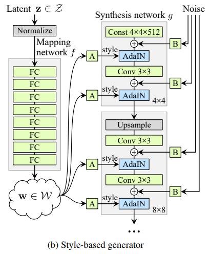
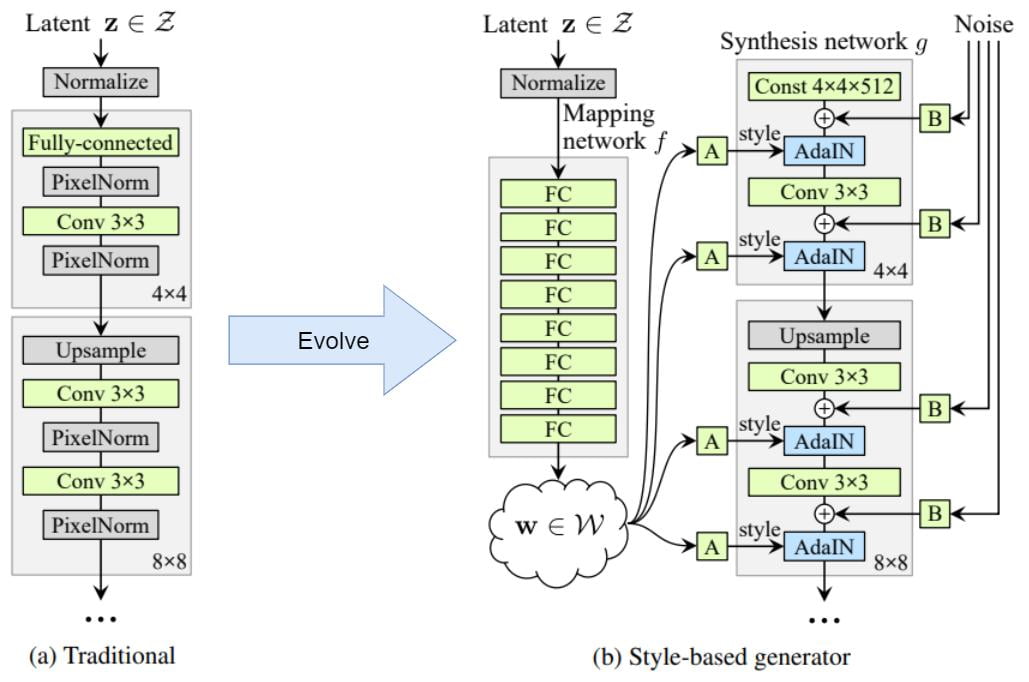
The architecture of the StyleGAN generator might look complicated at the first glance, but it actually evolved from ProGAN (Progressive GAN) step by step.

Step 1: Mapping and Styles

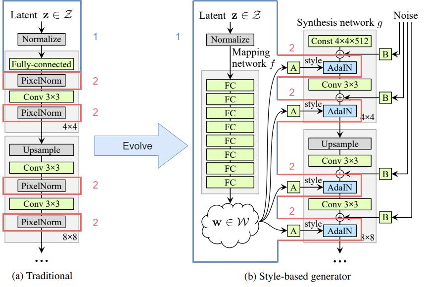
1. Instead of feeding the latent code \textbf{z} directly into the input layer, we feed it into a mapping network f to obtain a latent code \textbf{w}.
2. We then replace the PixelNorm with AdaIN (responsible for styling).
   

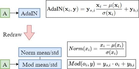
Let’s zoom into the styling module and see how AdaIN styles the intermediate feature map \textbf{x}_i. Here, \text{A} stands for a learned affine transformation.

The learned affine transformation \text{A} will transform the latent code \textbf{w} to style \textbf{y}. Hence, the feature map \textbf{x}_i is normalized by \mu and \sigma, and then denormalized by the style \textbf{y}.

I have explained how and why this will affect the style of the feature map/activation in my previous article, please read it if you want to understand better.

Step 2: Constant Input

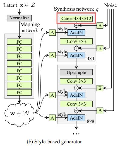
In traditional GAN, we input the latent code to the first layer of the synthesis network. In StyleGAN, we replace it with a constant vector.

We make a surprising observation that the network no longer benefits from feeding the latent code into the first convolution layer. We therefore simplify the architecture by removing the traditional input layer and starting the image synthesis from a learned 4 × 4 × 512 constant tensor.

It is found that the synthesis network can produce meaningful results even though it receives input only through the styles that control the AdaIN operations.

Step 3: Noise Inputs

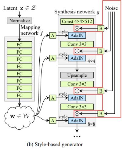
We then introduce explicit noise inputs for generating stochastic details (e.g. hairs, facial details). Here, \text{B} stands for a learned scaling factor.

The noise is broadcasted to all feature maps using learned per-feature scaling factors \text{B} and then added to the output of the corresponding convolution.

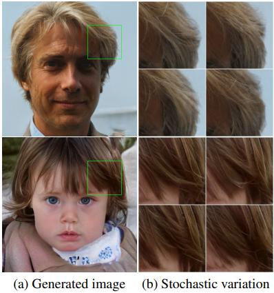
We can see that the noise affects only the stochastic aspects, leaving the overall composition and high-level aspects such as identity intact.

Step 4: Style Mixing

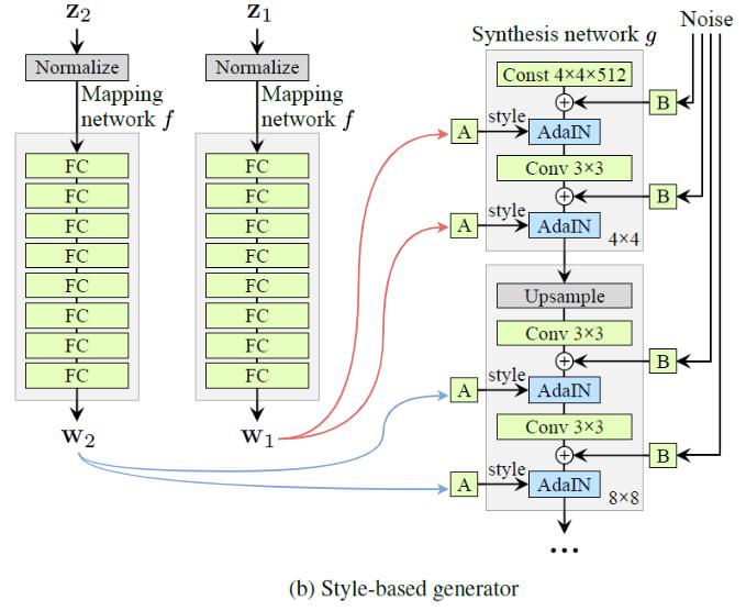
By employing mixing regularization, we can mix the styles of different latent codes.

To be specific, we run two latent codes \textbf{z}_1, \textbf{z}_2 through the mapping network, and have the corresponding \textbf{w}_1, \textbf{w}_2 control the styles so that \textbf{w}_1 applies before the crossover point and \textbf{w}_2 after it.

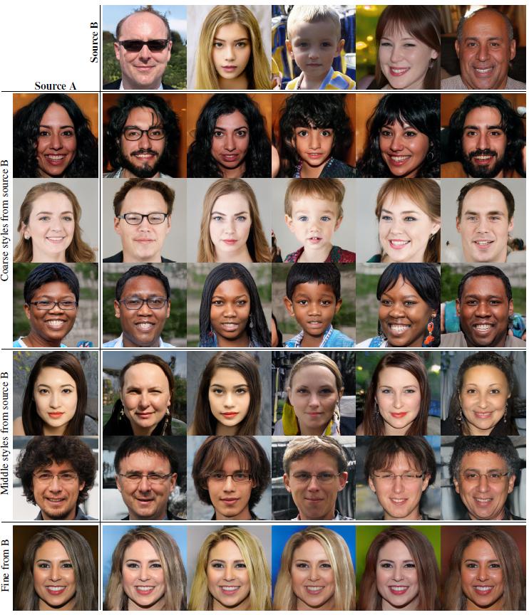
Two sets of images were generated from their respective latent codes (sources \text{A} and \text{B}); the rest of the images were generated by copying a specified subset of styles from source \text{B} and taking the rest from source \text{A}.

• Coarse: copying the styles of coarse resolutions (4×4 to 8×8) brings high-level aspects such as pose, general hairstyle, face shape, and eyeglasses from \text{B}, while all colors (eyes, hair, lighting) and finer facial features resemble \text{A}.
• Middle: copying the styles of middle resolutions (16×16 to 32×32) brings smaller scale facial features, hairstyle, eyes open/closed from \text{B}, while the pose, general face shape, and eyeglasses from A are preserved.
• Fine: copying the fine styles (64×64 to 1024×1024) from \text{B} brings mainly the color scheme and microstructure.

StyleGAN2

The main purpose of StyleGAN2 is to tackle the water-droplet artifacts that appeared in StyleGAN images.

Reason

The researchers pinpointed the problem to the AdaIN operation.

Before we talk about it, let’s break down the AdaIN operation into two parts: Normalization and Modulation.

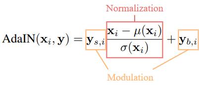
It is found that when the Normalization step is removed from the generator, the droplet artifacts disappear completely.

The researchers then hypothesize that the droplet artifact is a result of the generator intentionally sneaking signal strength information passing through the instance normalization step of AdaIN.

Hypothesis:

By creating a strong, localized spike that dominates the statistics, the generator can effectively scale the signal as it likes elsewhere.

Original StyleGAN Design

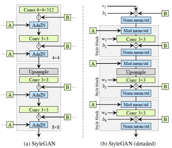
The above diagram is simply the architecture of the original StyleGAN generator. We redrew the diagram by breaking down the AdaIN operation into Norm mean/std and Mod mean/std (Normalization and Modulation).

In addition, we explicitly annotated the learned weights (w), biases (b), and the constant input (c) on the diagram. Also, we redrew the gray boxes so that only one style is active per box.

Changes #1

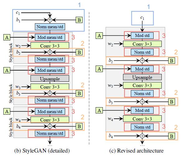
1. We removed some redundant operations at the beginning.
2. We moved the addition of b and \text{B} to be outside the active area of style (we observed that more predictable results are obtained by doing this).
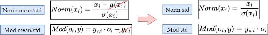
3. It is sufficient for the normalization and modulation to operate on the standard deviation alone (i.e. the mean is not needed).

Changes #2

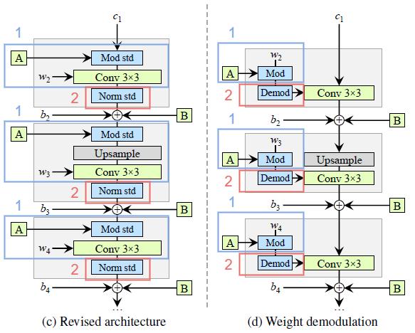
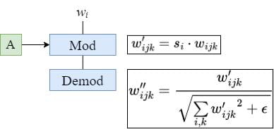
1. We combine the Mod std and Conv operations to be w_{ijk}' = s_i \cdot w_{ijk}.
2. We change Norm std to become weight demodulation.

Combine Mod std and Conv

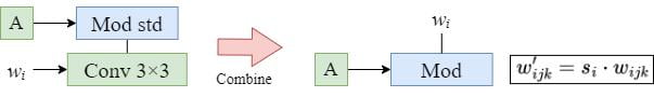
The reason why we can combine the Mod std and Conv is that their effect is:

The modulation scales each input feature map of the convolution based on the incoming style, which can alternatively be implemented by scaling the convolution weights: w_{ijk}' = s_i \cdot w_{ijk}.

• w: original weights
• w': modulated weights
• s_i: the scale corresponding to the ith input feature map
• j, k: spatial indices of the output feature maps

Weight Demodulation

The purpose of instance normalization is to essentially remove the effect of s from the statistics of the convolution’s output feature maps (see the above figure).

If the input activations are distributions with unit standard deviation (sd=1), the standard deviation of the output activations will be:

\sigma_j = \sqrt{\sum_{i,k} {w_{ijk}'}^2}

The standard deviation of the output activations after modulation and convolution

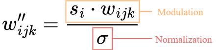
Therefore, w_{ijk}' is normalized (demodulated) as follows:

w_{ijk}'' = w_{ijk}' \bigg/ \sqrt{\sum_{i,k} {w_{ijk}'}^2 + \epsilon}

where \epsilon is a small constant to avoid numerical issues (for stability)

All in all, the new Mod and Demod operations look like this:

Changes #3

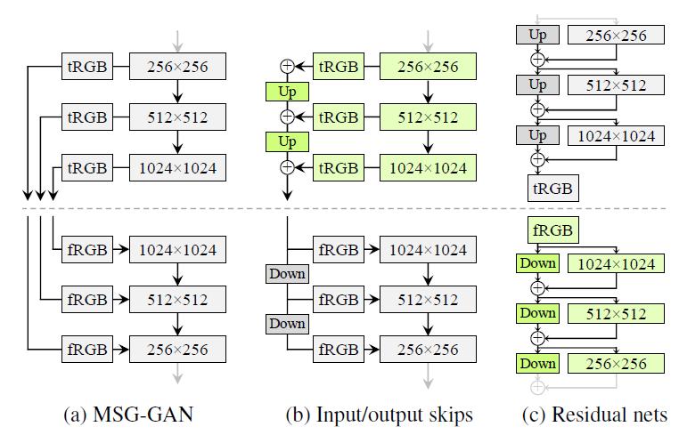
Instead of using the progressive growth method, StyleGAN2 explores skip connections and ResNets design to produce high-quality images.

Up and Down denote bilinear up and down-sampling respectively. tRGB and fRGB represent “to RGB” and “from RGB” respectively.

StyleGAN2 Results

As a result, replacing normalization with demodulation removes the characteristic artifacts from images and activations. This is because:

Compared to instance normalization, our demodulation technique is weaker because it is based on statistical assumptions about the signal instead of actual contents of the feature maps.

StyleGAN2-ADA

The purpose of StyleGAN2-ADA is to design a method to train GAN with limited data, where ADA stands for Adaptive Discriminator Augmentation.

Stochastic Discriminator Augmentation

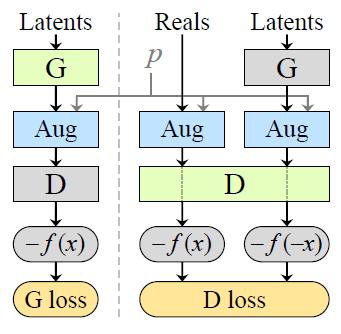
\text{G} and \text{D} stand for the generator and discriminator respectively.

Where p \in [0, 1] is the augmentation probability that controls the strength of the augmentations.

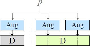
The discriminator \text{D} rarely sees a clean image because

• We have many augmentations in the pipeline
• The value of p will be set around 0.8

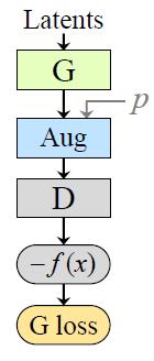
The generated images will be augmented before being evaluated by the discriminator \text{D} during training. Since the Aug operation is being put after the generation, the generator \text{G} is guided to produce only clean images.

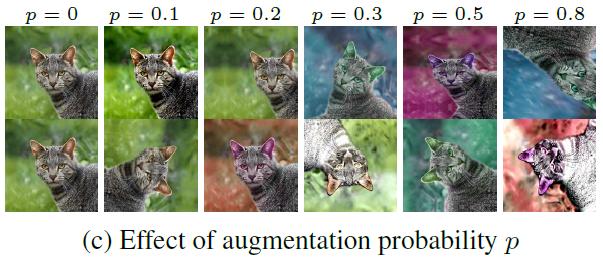
From the experiment, it is found that the following 3 types of augmentations are the most effective:

• pixel blitting (x-flips, 90° rotations, integer translation)
• geometric
• color transforms
  

Adaptive Discriminator Augmentation

In the previous stochastic discriminator augmentation setup, we used the same value of p for all the transformations. However, we would like to avoid manual tuning of the augmentation strength p and instead control it dynamically based on the degree of overfitting.

Let’s denote \text{D}_\text{train}, \text{D}_\text{validation}, \text{D}_\text{generated}, and \text{D}_\text{real} as the discriminator outputs of the training set, validation set, generated images, and testing set respectively.

The researchers designed the following heuristics to quantify overfitting.

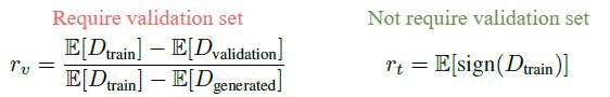
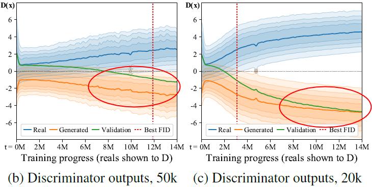
Heuristic #1: r_v

Idea: Since the training set and the validation set are simply split sets from the real images, \text{D}_\text{validation} should be closer to \text{D}_\text{real} / \text{D}_\text{train} ideally. However, when it overfits, the \text{D}_\text{validation} (green) will get closer to \text{D}_\text{generated} (orange).

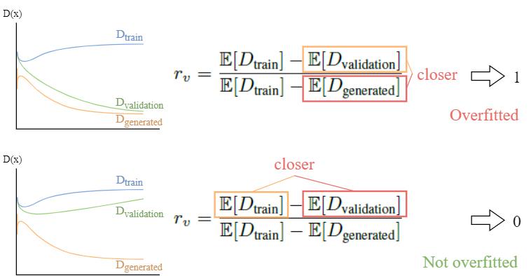
The drawback of this heuristic is that it requires a validation set. Since we already have so little data, we don’t want to further split the dataset. Therefore, we include it mainly as a comparison method.

Heuristic #2: r_t

In training, we will use the second heuristic r_t.

Idea: \text{D}_\text{real} / \text{D}_\text{train} and \text{D}_\text{generated} diverge symmetrically around zero when the situation gets worse (overfitting).

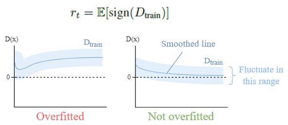
r_t estimates the portion of the \text{D}_\text{train} getting a positive value. If \text{D}_\text{train} diverges from zero, it is overfitting; otherwise, it is not overfitting.

Adjust p Using r_t

1. Initialize p = 0
2. Adjust p every 4 mini-batches based on the following conditions:

• If r_t is high → overfitting → increase p (augment more)
• If r_t is low → not overfitting → decrease p (augment less)

StyleGAN2-ADA Results

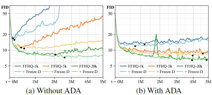
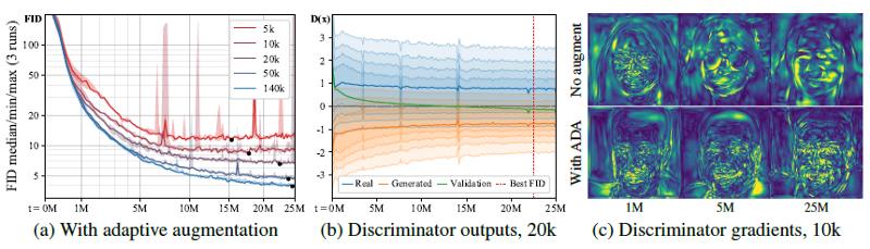
(a) Training curves for FFHQ with different training set sizes using adaptive augmentation.

(b) The supports of real generated images continue to overlap.

(c) Example magnitudes of the gradients the generator receives from the discriminator as the training progresses.

StyleGAN3

The remaining parts are the main points that I summarized in my previous article: “StyleGAN3 Clearly Explained!”. If you want to know the details of StyleGAN3, please directly go to this link and continue reading about it.

The purpose of StyleGAN3 is to tackle the “texture sticking” issue that happened in the morphing transition (e.g. morphing from one face to another face).

In other words, StyleGAN3 tries to make the transition animation more natural.

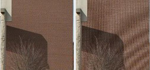
Texture Sticking

As you can see from the above animations, the beard and hair (left) look like sticking to the screen when morphing, while the one generated by StyleGAN3 (right) does not have this sticky pixels problem.

Reason: Positional References

It turns out that there are some unintentional positional references available in the intermediate layers for the network to process feature maps through the following sources:

• Image borders
• Per-pixel noise inputs
• Positional encodings
• Aliasing

These positional references make the network generates pixels sticking to the same coordinates.

Among them, aliasing is the hardest one to identify and fix.

Aliasing

Aliasing is an effect that causes different signals to become indistinguishable (or aliases of one another) when sampled.

It also often refers to the distortion or artifact that results when a signal reconstructed from samples is different from the original continuous signal.

E.g. When we sample a high-frequency signal (e.g. the blue sine wave), if it results in a lower frequency signal (the red wave), then this is called aliasing. This happens because the sampling rate is too low.

The researchers have identified two sources for aliasing in GAN:

1. Faint after-images of the pixel grid resulting from non-ideal upsampling filters (e.g. nearest, bilinear, or stridden convolutions)
2. The pointwise application of nonlinearities (e.g. ReLU, or swish)

Even with a small amount of aliasing, it is amplified throughout the network and becomes a fixed position in the screen coordinates.

Goal

The goal is to eliminate all sources of positional references. After that, the details of the images can be generated equally well regardless of pixel coordinates.

In order to remove positional references, the paper proposed to make the network equivariant:

Consider an operation f (e.g. convolution, upsampling, ReLU, etc.) and a spatial transformation t (e.g. translation, rotation).

f is equivariant with respect to t if t \circ f = f \circ t.

In other words, an operation (e.g. ReLU), should not insert any positional codes/references which will affect the transformation procedure, and vice versa.

Redesigning Network Layers

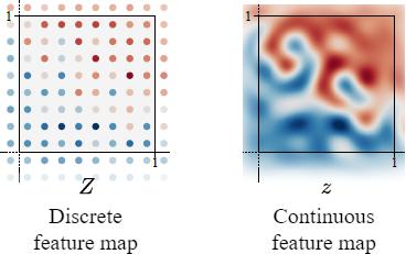
Practical neural networks operate on discretely sampled feature maps. It is found that we need the network to operate in the continuous domain to efficiently suppress the aliasing problem. Therefore, we have to redesign the network layers (i.e. convolution, upsampling/downsampling, nonlinearity).

The details of how to redesign the network layers are too long and I am not going to include them here. I have explained them in “StyleGAN3 Clearly Explained!”.

If you didn’t read it, never mind. All you need to know is that by redesigning the network layers to operate on continuous feature maps (continuous signals), aliasing can be suppressed.

Changes

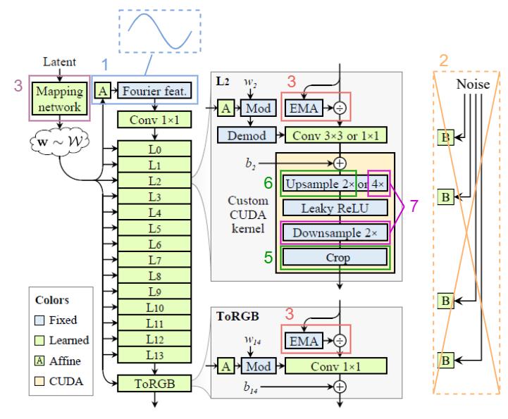
1. Replaced the learned input constant in StyleGAN2 with the Fourier feature to facilitate exact continuous translation and rotation of z.
2. Removed the per-pixel noise inputs to eliminate positional references introduced by them.
3. Decreased the mapping network depth to simplify the setup.
4. Eliminated the output skip connections (which were used to deal with the gradient vanishing problem. We address that by using a simple normalization before each convolution, i.e. divided by EMA: Exponential Moving Average)
5. Maintained a fixed-size margin around the target canvas, cropping to this extended canvas after each layer (to leak absolute image coordinates into internal representations, because the signals outside the canvas are also important).
6. Replaced the bilinear 2× upsampling filter with a better approximation of the ideal low-pass filter.
7. Motivated by our theoretical model, we wrap the leaky ReLU between m×upsampling and m×downsampling. (we can fuse the previous 2×upsampling with this m×upsampling, i.e. choose m=2, then we have 4×upsampling before each leaky ReLU)

Note: the network layers (i.e. convolution, up/downsampling, ReLU) are replaced with the corresponding redesigned layers.

StyleGAN3 Results

The alias-free translation (middle) and rotation (bottom) equivariant networks build the image in a radically different manner from what appear to be multi-scale phase signals that follow the features seen in the final image.

In the internal representations, it looks like a new coordinate system is being invented and details are drawn on these surfaces.

Summary

The purposes of each of them:

• StyleGAN: to generate high-fidelity images.
• StyleGAN2: to remove water-droplet artifacts in StyleGAN.
• StyleGAN2-ADA: to train StyleGAN2 with limited data.
• StyleGAN3: to make transition animation more natural.

References

[1] T. Karras, S. Laine and T. Aila, “A Style-Based Generator Architecture for Generative Adversarial Networks”, arXiv.org, 2022. https://arxiv.org/abs/1812.04948

[2] T. Karras, S. Laine, M. Aittala, J. Hellsten, J. Lehtinen and T. Aila, “Analyzing and Improving the Image Quality of StyleGAN”, arXiv.org, 2022. https://arxiv.org/abs/1912.04958

[3] T. Karras, M. Aittala, J. Hellsten, S. Laine, J. Lehtinen and T. Aila, “Training Generative Adversarial Networks with Limited Data”, arXiv.org, 2022. https://arxiv.org/abs/2006.06676

[4] T. Karras et al., “Alias-Free Generative Adversarial Networks”, arXiv.org, 2022. https://arxiv.org/abs/2106.12423

[5] “Aliasing — Wikipedia”, En.wikipedia.org, 2022. https://en.wikipedia.org/wiki/Aliasing