MMDiT Joint Attention in PyTorch: Two Streams, One Generator
Where you are: Post 13 of 14 in PyTorch Tutorial 2026 · about 10 min read
What you’ll build: An MMDiT-style TinyDiT: condition tokens, the joint-attention double-stream block, single-stream blocks after it, and a size-matched before/after.
You’ll need: Post 11 (2D RoPE, QK-norm) and Post 12 (adaLN-Zero, label dropout, guidance).
In this post:
- Introduction
- Step 1/5: Three Ways to Feed a Condition
- Step 2/5: Condition Tokens
- Step 3/5: The Double-Stream Block
- Step 4/5: Double-Stream, Then Single-Stream
- Step 5/5: The Before/After on TinyDiT
- Recap
Series: PyTorch Tutorial 2026 (14 posts)
- Post 1: PyTorch Tutorial 2026: From Tensors to Tiny Diffusion
- Post 2: PyTorch Tensors Explained: Shapes, Broadcasting, and Images as Arrays
- Post 3: PyTorch Autograd: How backward() Builds Gradients
- Post 4: PyTorch DataLoader Explained: Datasets, Batches, and Image Folders
- Post 5: PyTorch nn.Module and the Training Loop: Layers, Loss, and Checkpoints
- Post 6: Attention and the Transformer Block in PyTorch
- Post 7: Patch Embeddings in PyTorch: How a Transformer Reads an Image
- Post 8: Flow Matching in PyTorch: Train a Model to Follow a Straight Line
- Post 9: Build a Tiny Diffusion Transformer in PyTorch (DiT from Scratch)
- Post 10: torch.compile, Mixed Precision, and SDPA: Speed Up TinyDiT
- Post 11: RMSNorm, QK-Norm, SwiGLU, and 2D RoPE in a Tiny DiT
- Post 12: adaLN-Zero and Classifier-Free Guidance in PyTorch
- Post 13: MMDiT Joint Attention in PyTorch: Two Streams, One Generator (you are here)
- Post 14: Train and Sample Like 2026: Logit-Normal Steps, EMA, and Few-Step Flow
Introduction
In adaLN-Zero and Classifier-Free Guidance in PyTorch the class label was squeezed into one vector and added to the time signal. That works for 10 classes. It doesn’t work for “a red fox jumping over a frozen river at sunset”: a prompt is many tokens, and a single vector loses most of it.
Stable Diffusion 3 (Esser et al., Scaling Rectified Flow Transformers for High-Resolution Image Synthesis, 2024) and FLUX solved this with the Multimodal Diffusion Transformer (MMDiT). The prompt tokens and the image tokens go through the transformer together, in one joint attention.
In this MMDiT PyTorch tutorial we build the joint-attention block, the “double-stream” and “single-stream” designs, and test them on TinyDiT with class labels standing in for text.
Note: CPU settings used in this post: dim 128, 4 heads, 2D RoPE and QK-norm (post 11), adaLN-Zero (post 12), class-conditional with 10% label dropout, batch 128, 3,000 steps per run on an 8-core CPU.
Watch out: We have no text encoder on a CPU budget, so each class is represented by 4 learned “condition tokens”. The mechanics are exactly the same as with text tokens, but don’t expect a 10-class toy to show the benefits MMDiT has for long prompts.
Step 1/5: Three Ways to Feed a Condition
In this step: We compare adaLN, cross-attention and joint attention, the three ways a diffusion transformer can read a condition.
| Method | Where the condition goes | Used by |
|---|---|---|
| adaLN (posts 9 and 12) | one vector, scales and shifts every LayerNorm | DiT (class labels), also for the time signal in SD3 and FLUX |
| Cross-attention | image tokens attend to text tokens in a separate attention layer | Stable Diffusion 1 and 2, PixArt |
| Joint attention (MMDiT) | text and image tokens are concatenated and attend to each other in one attention | SD3, FLUX |
With cross-attention the text is read-only: images look at text, text never updates. With joint attention, information flows both ways in every layer: the text tokens are updated by what the image looks like, too.
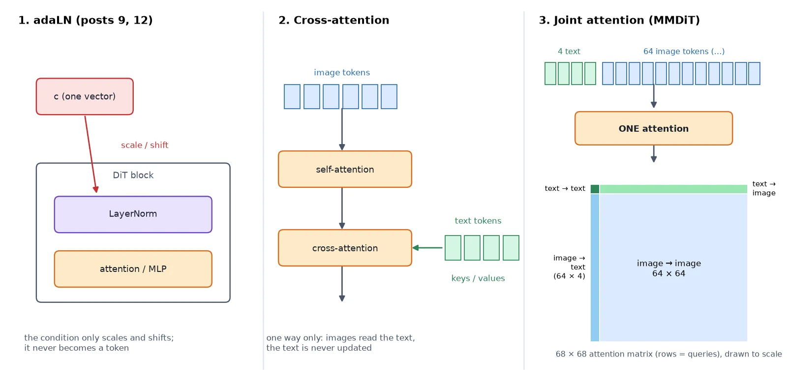
What you just built: A map of the three conditioning methods, and why joint attention is the one that lets information flow both ways.
Step 2/5: Condition Tokens
In this step: We represent each class as 4 learned tokens and join them with the 64 image tokens into one sequence.
Our “prompt” is a class id, so we give each class a small set of learned tokens: an nn.Embedding(11, 4 × D) reshaped to 4 tokens of size D. It has 11 rows again, with the “no label” row for CFG. With real text, these would be the outputs of a text encoder like T5 or CLIP.
import torch
from tinydit.expert import ExpertConfig, ExpertTinyDiT

torch.manual_seed(0)
cfg = ExpertConfig(dim=128, depth=4, num_heads=4, class_cond=True, cond_mode="joint", cond_tokens=4, double_blocks=2)
model = ExpertTinyDiT(cfg)
x, t, y = torch.randn(2, 3, 32, 32), torch.rand(2), torch.tensor([3, 10])
ctx = model.ctx_embed(y).view(2, cfg.cond_tokens, cfg.dim)
print("condition tokens:", tuple(ctx.shape), " image tokens:", (2, 64, 128))
print("joint sequence  :", (2, cfg.cond_tokens + 64, 128), "-> attention matrix", (cfg.cond_tokens + 64,) * 2, "per head")
print("blocks:", [type(b).__name__ for b in model.joint_blocks] + [type(b).__name__ for b in model.blocks])
print("output:", tuple(model(x, t, y).shape))condition tokens: (2, 4, 128) image tokens: (2, 64, 128)
joint sequence : (2, 68, 128) -> attention matrix (68, 68) per head
blocks: ['DoubleStreamBlock', 'DoubleStreamBlock', 'ExpertDiTBlock', 'ExpertDiTBlock']
output: (2, 3, 32, 32)64 image tokens plus 4 condition tokens make a joint sequence of 68, and each head’s attention matrix is 68 × 68.
Condition tokens: what, why, how
What it is: the condition represented as a sequence of tokens instead of one vector.
Why it works: a sequence can carry much more information than one vector, and attention can pick out the part each image patch needs.
How it works: for class labels: nn.Embedding(classes + 1, K * D) reshaped to (N, K, D). For text: the token outputs of a text encoder, projected to width D.
What you just built: Condition tokens: 4 learned tokens per class (plus “no label”), joined with the image tokens into a 68-token sequence.
Step 3/5: The Double-Stream Block
In this step: We build the SD3-style block: separate weights for each kind of token, one shared attention over both.
Text and image tokens are different kinds of thing, so SD3 gives them separate weights: each stream has its own norms, its own QKV and output projections, and its own MLP. Only the attention is shared:
- Each stream computes its own q, k, v (with its own adaLN modulation from the time vector).
- Concatenate: q = [q_{\text{txt}}; q_{\text{img}}], same for k and v.
- One attention over all 68 tokens.
- Split the output back into the two streams; each continues with its own projection and MLP.
\begin{aligned} q &= [\,q_{\text{txt}};\, q_{\text{img}}\,] \quad \text{(68 rows; the same for } k \text{ and } v) \\ \text{out} &= \operatorname{softmax}\!\big(q\,k^\top / \sqrt{d}\big)\, v \quad (68 \times 68 \text{ scores per head}) \\ [\,\text{out}_{\text{txt}};\, \text{out}_{\text{img}}\,] &= \text{split}(\text{out},\; 4 + 64) \end{aligned}The constructor reuses two post-12 blocks, one per stream, and reads each stream’s modulation vectors:
class DoubleStreamBlock(nn.Module):
    """MMDiT block (SD3; FLUX.1 'double' block): image tokens and condition tokens keep their own
    norms, QKV/out projections and MLPs, but attend jointly over the concatenated sequence."""

    def __init__(self, cfg: ExpertConfig):
        super().__init__()
        self.img = ExpertDiTBlock(cfg)         # reuse: norms, attn (qkv + proj), mlp, adaLN for the image stream
        self.txt = ExpertDiTBlock(cfg)         # same pieces for the condition stream
        self.zero = cfg.adaln_zero

    def _mods(self, block, c):
        if self.zero:
            return block.adaLN(c)[:, None].chunk(6, dim=-1)
        sh1, sc1, sh2, sc2 = block.adaLN(c)[:, None].chunk(4, dim=-1)
return sh1, sc1, 1.0, sh2, sc2, 1.0The forward pass is where the streams meet: concatenate, one attention, split back:
    def forward(self, x: torch.Tensor, ctx: torch.Tensor, c: torch.Tensor, rope=None):
        mi, mt = self._mods(self.img, c), self._mods(self.txt, c)
        qi, ki, vi = self.img.attn.qkv_heads(self.img.norm1(x) * (1 + mi[1]) + mi[0])
        qt, kt, vt = self.txt.attn.qkv_heads(self.txt.norm1(ctx) * (1 + mt[1]) + mt[0])
        q, k, v = (torch.cat([a, b], dim=2) for a, b in ((qt, qi), (kt, ki), (vt, vi)))   # concat: [ctx, img]
        if rope is not None:
            q, k = apply_rope(q, *rope), apply_rope(k, *rope)
        out = self.img.attn.attend(q, k, v)                       # ONE attention over both streams
        n_ctx = ctx.shape[1]
        out_t, out_i = out[:, :n_ctx], out[:, n_ctx:]             # split back
        x = x + mi[2] * self.img.attn.proj(out_i)
        ctx = ctx + mt[2] * self.txt.attn.proj(out_t)
        x = x + mi[5] * self.img.mlp(self.img.norm2(x) * (1 + mi[4]) + mi[3])
        ctx = ctx + mt[5] * self.txt.mlp(self.txt.norm2(ctx) * (1 + mt[4]) + mt[3])
return x, ctxLook how much we reuse: each stream is just an ExpertDiTBlock from post 12, used for its parts.
Note: With RoPE (post 11), the condition tokens get angle 0 (no position), and image tokens rotate as before.
Double-stream (MMDiT) block: what, why, how
What it is: a block that lets image and condition tokens exchange information in every layer, while keeping separate weights for each modality.
Why it works: joint attention gives two-way information flow (text ↔ image), and separate weights let each modality keep its own feature statistics (SD3, 2024).
How it works: per stream: adaLN-modulated norm → QKV. Concatenate q, k, v across streams, one attention, split, then per-stream output projection and MLP with gates.
What you just built: DoubleStreamBlock: two sets of weights, one joint attention over 68 tokens.
Step 4/5: Double-Stream, Then Single-Stream
In this step: We add cheaper single-stream blocks after the double-stream ones, the way FLUX.1 does, and count the parameters.
Two sets of weights per block costs parameters. FLUX.1 uses a mix: a number of double-stream blocks first, then single-stream blocks that simply run a normal transformer block on the concatenated sequence (shared weights for both kinds of token).
Our ExpertTinyDiT supports both with one setting, double_blocks:
from tinydit.expert import ExpertConfig, ExpertTinyDiT

base = dict(dim=128, num_heads=4, class_cond=True, adaln_zero=True)
setups = {
    "adaLN-Zero, 4 single blocks (post 12)": dict(depth=4),
    "joint, 2 double + 2 single (MMDiT/FLUX-style)": dict(depth=4, cond_mode="joint", double_blocks=2),
    "joint, 4 double (SD3-style)": dict(depth=4, cond_mode="joint", double_blocks=4),
}
for name, extra in setups.items():
    m = ExpertTinyDiT(ExpertConfig(**base, **extra))
print(f"{name:46s} {sum(p.numel() for p in m.parameters()):>10,d} parameters")adaLN-Zero, 4 single blocks (post 12) 1,285,680 parameters
joint, 2 double + 2 single (MMDiT/FLUX-style) 1,883,568 parameters
joint, 4 double (SD3-style) 2,477,232 parametersWatch out: Double-stream blocks nearly double the block’s parameters. So a fair comparison must also include a plain adaLN-Zero model made bigger to the same size. Otherwise “joint attention is better” might only mean “more parameters is better”.
Our param-matched baseline is the post-12 model with 6 blocks instead of 4.
Single-stream block: what, why, how
What it is: cheaper joint layers after the double-stream ones.
Why it works: once the two kinds of token have been mixed for a few layers, sharing weights saves parameters (FLUX.1 uses many single-stream blocks after its double-stream ones).
How it works: h = cat([ctx, img]) then ordinary ExpertDiTBlocks, then drop the condition tokens before the final layer.
What you just built: An ExpertTinyDiT with double_blocks=2 (2 double-stream, then 2 single-stream blocks), and a same-size 6-block baseline to compare against.
Step 5/5: The Before/After on TinyDiT
In this step: We train three class-conditional models and compare quality, label following and speed.
Three class-conditional runs with the same seed, steps and settings:
- the post-12 adaLN-Zero model;
- the same model with 6 blocks, so it has the same size as the joint model;
- the joint model (2 double-stream blocks, then 2 single-stream blocks).
Scores are for the trained weights, at three guidance scales:
import json
from pathlib import Path

def load(name):
    return json.loads(Path(f"../runs/{name}/metrics.json").read_text())

runs = {"adaLN-Zero, 4 blocks (post 12)": "p12_cond_zero",
        "adaLN-Zero, 6 blocks (same size)": "p13_zero_d6",
        "joint: 2 double + 2 single": "p13_joint22"}
print(f"{'model':33s} {'params':>9s} {'val MSE':>8s} | probe-FD / class acc at guidance w = 1, 1.5, 3")
for name, run in runs.items():
    m = load(run); r = m["raw"]                   # trained weights, no EMA, same seed and steps
    scores = "  ".join(f"{r[f'cfg{w}']['probe_fd']:5.1f} / {r[f'cfg{w}']['probe_acc']:5.1%}" for w in ("1.0", "1.5", "3.0"))
print(f"{name:33s} {m['params']:9,d} {r['val_mse']:8.4f} | {scores}")model params val MSE | probe-FD / class acc at guidance w = 1, 1.5, 3
adaLN-Zero, 4 blocks (post 12) 1,283,888 0.2157 | 53.2 / 25.3% 50.3 / 32.7% 52.3 / 45.2%
adaLN-Zero, 6 blocks (same size) 1,877,680 0.2120 | 49.1 / 29.9% 47.4 / 37.0% 48.5 / 49.4%
joint: 2 double + 2 single 1,881,904 0.2128 | 44.9 / 25.8% 41.2 / 34.0% 33.3 / 50.8%| Model | Params | Val MSE | Probe-FD (w = 1.5) | Class acc (w = 1.5) | Probe-FD (w = 3) | Class acc (w = 3) |
|---|---|---|---|---|---|---|
| adaLN-Zero, 4 blocks (post 12) | 1.28M | 0.2157 | 50.3 | 32.7% | 52.3 | 45.2% |
| adaLN-Zero, 6 blocks (same size) | 1.88M | 0.2120 | 47.4 | 37.0% | 48.5 | 49.4% |
| Joint attention (MMDiT-style) | 1.88M | 0.2128 | 41.2 | 34.0% | 33.3 | 50.8% |
What the numbers say:
- The size-matched baseline matters. Going from 4 to 6 adaLN-Zero blocks improved everything a bit (val MSE 0.2157 → 0.2120, probe-FD 50.3 → 47.4). Comparing the joint model only with the 4-block model would have given joint attention credit for those gains too.
- Against the same-size model, joint attention made clearly better samples. Probe-FD dropped from 47.4 to 41.2 at w = 1.5, and from 48.5 to 33.3 at w = 3. That last one is the best probe-FD in the whole series so far.
- Guidance behaved differently. Guidance kept improving the joint model’s probe-FD up to w = 3, while the adaLN models got worse past 1.5.
- But it didn’t follow the label better. Val MSE is the same (0.2128 vs 0.2120, inside seed noise), and at low guidance the joint model’s class accuracy is a little lower (34.0% vs 37.0% at w = 1.5). At w = 3 the two are about level (50.8% vs 49.4%).
Why it works: With one label as the condition, joint attention mainly bought us better image quality per parameter, not better label following. That fits the design. MMDiT’s big advantage is reading long conditions like prompts, where squeezing everything into one adaLN vector loses information. A class label is already one vector, so there’s little left to gain on that side.
Watch out: It’s one seed per model, so treat differences of a point or two as noise; the probe-FD gap at w = 3 is far bigger than that.
Training cost
The steps-per-second numbers in the run logs were measured while other runs shared the CPU. So here is a fair timing, the three models taking turns in one process:
import time
import torch
from tinydit.expert import ExpertConfig, ExpertTinyDiT
from tinydit.flow import FlowMatchingLoss

torch.manual_seed(0)
torch.set_num_threads(2)
x, y = torch.randn(64, 3, 32, 32), torch.randint(0, 10, (64,))
base = dict(dim=128, num_heads=4, pos="rope2d", qk_norm=True, class_cond=True, adaln_zero=True)
variants = {"adaLN-Zero, 4 blocks": dict(depth=4), "adaLN-Zero, 6 blocks": dict(depth=6),
            "joint, 2 double + 2 single": dict(depth=4, cond_mode="joint", double_blocks=2)}
models = {k: ExpertTinyDiT(ExpertConfig(**base, **v)) for k, v in variants.items()}
opts = {k: torch.optim.AdamW(m.parameters(), lr=3e-4) for k, m in models.items()}
loss_fn = FlowMatchingLoss(conditional=True, drop_prob=0.1, null_class=10)
times = {k: [] for k in models}
for rnd in range(12):                  # take turns, so background load slows every model equally
    for name, model in models.items():
        t0 = time.perf_counter()
        opts[name].zero_grad()
        loss_fn(model, (x, y)).backward()
        opts[name].step()
        if rnd >= 2:
            times[name].append(time.perf_counter() - t0)
for name, ts in times.items():
print(f"{name:27s} {sorted(ts)[5] * 1000:6.1f} ms per training step (batch 64, median of 10)")adaLN-Zero, 4 blocks 192.9 ms per training step (batch 64, median of 10)
adaLN-Zero, 6 blocks 299.6 ms per training step (batch 64, median of 10)
joint, 2 double + 2 single 214.6 ms per training step (batch 64, median of 10)The joint model has the same parameters as the 6-block model but trains about 28% faster per step (215 vs 299 ms). Its extra weights belong to the condition stream, which only handles 4 tokens, so they add little compute. Compared with the 4-block model it costs about 12% more time per step for the best probe-FD so far.
What you just built: A measured before/after: joint attention gives the best probe-FD so far (41.2 at w = 1.5, 33.3 at w = 3) at the same size as a 6-block model, and trains 28% faster per step than it.
Recap
- MMDiT joint attention (SD3, FLUX) puts the condition tokens and image tokens into one sequence and runs one attention over both, so information flows both ways in every layer.
- A double-stream block keeps separate norms, projections and MLPs for each kind of token and only shares the attention. A single-stream block is an ordinary block run over the joined sequence. FLUX.1 uses double-stream blocks first, then single-stream ones, and so does our TinyDiT with
double_blocks=2. - For class labels we used 4 learned condition tokens per class; with text they’d come from a text encoder.
- Double-stream blocks add a lot of parameters, so we compared against a same-size adaLN-Zero model (6 blocks). Against it, joint attention gave much better probe-FD (41.2 vs 47.4 at w = 1.5, 33.3 vs 48.5 at w = 3) but the same val MSE and similar class accuracy.
- With a single class label, the gain is in image quality, not label following. The bigger benefit of MMDiT, reading long prompts, is something a 10-class toy can’t show.
Next up: The last post, Train and Sample Like 2026: Logit-Normal Steps, EMA, and Few-Step Flow: the training and sampling tricks of 2026, logit-normal timesteps, EMA weights and rectified-flow reflow for few-step sampling, then a final side-by-side of the simple and the expert TinyDiT.
Series: PyTorch Tutorial 2026 (14 posts)
- Post 1: PyTorch Tutorial 2026: From Tensors to Tiny Diffusion
- Post 2: PyTorch Tensors Explained: Shapes, Broadcasting, and Images as Arrays
- Post 3: PyTorch Autograd: How backward() Builds Gradients
- Post 4: PyTorch DataLoader Explained: Datasets, Batches, and Image Folders
- Post 5: PyTorch nn.Module and the Training Loop: Layers, Loss, and Checkpoints
- Post 6: Attention and the Transformer Block in PyTorch
- Post 7: Patch Embeddings in PyTorch: How a Transformer Reads an Image
- Post 8: Flow Matching in PyTorch: Train a Model to Follow a Straight Line
- Post 9: Build a Tiny Diffusion Transformer in PyTorch (DiT from Scratch)
- Post 10: torch.compile, Mixed Precision, and SDPA: Speed Up TinyDiT
- Post 11: RMSNorm, QK-Norm, SwiGLU, and 2D RoPE in a Tiny DiT
- Post 12: adaLN-Zero and Classifier-Free Guidance in PyTorch
- Post 13: MMDiT Joint Attention in PyTorch: Two Streams, One Generator (you are here)
- Post 14: Train and Sample Like 2026: Logit-Normal Steps, EMA, and Few-Step Flow
← Previous: Post 12: adaLN-Zero and Classifier-Free Guidance in PyTorch
Next → Post 14: Train and Sample Like 2026: Logit-Normal Steps, EMA, and Few-Step Flow