torch.compile, Mixed Precision, and SDPA: Speed Up TinyDiT

In this post:

• Introduction
• Step 1/6: SDPA: The Attention Kernel PyTorch Ships
• Step 2/6: Mixed Precision: autocast, bfloat16 and the GradScaler
• Step 3/6: torch.compile: Turning Python into Fused Kernels
• Step 4/6: FastTrainer: Three Switches, Same Trainer
• Step 5/6: The Benchmark: What Actually Got Faster?
• Step 6/6: One Command per Experiment
• Recap

Introduction

TinyDiT works, but it took 11 minutes for 6,000 steps on a CPU, and the Expert posts will train it again and again. So before we upgrade the model, let’s upgrade the training loop with the three speed tools PyTorch 2 is known for: F.scaled_dot_product_attention (SDPA), mixed precision with torch.autocast, and torch.compile.

We’ll add them to our trainer as simple on/off switches, check that the results don’t change, and then time every combination. Some of the results surprised me, and I’ll show you all of them, including the ones where a “speed-up” made things slower.

In Build a Tiny Diffusion Transformer in PyTorch (DiT from Scratch) we assembled and trained TinyDiT with the plain post-5 Trainer. Today’s FastTrainer is that same trainer with two extra options, and nothing else about the model or the loss changes.

Step 1/6: SDPA: The Attention Kernel PyTorch Ships

In this step: We switch our hand-written attention to PyTorch’s fused F.scaled_dot_product_attention and time the difference.

In post 6 we wrote attention by hand, softmax(q @ k.T / sqrt(d)) @ v, and promised to switch to F.scaled_dot_product_attention later. It computes exactly the same thing, but as one fused operation.

On a GPU it can dispatch to FlashAttention (Dao et al., 2022), which never stores the full L \times L attention matrix, so it’s faster and uses far less memory. Let’s check that it’s the same math, and time one attention call.

First, the same inputs through both versions:

import time
import torch
import torch.nn.functional as F
from tinydit.attention import attention

torch.manual_seed(0)
q, k, v = (torch.randn(128, 4, 64, 32, requires_grad=True) for _ in range(3))   # (N, heads, L, head_dim)

out_manual, _ = attention(q, k, v)                     # post 6: softmax(q k^T / sqrt(d)) v, by hand
out_sdpa = F.scaled_dot_product_attention(q, k, v)      # PyTorch's fused version
print("same result:", torch.allclose(out_manual, out_sdpa, atol=1e-5))

import time
import torch
import torch.nn.functional as F
from tinydit.attention import attention

torch.manual_seed(0)
q, k, v = (torch.randn(128, 4, 64, 32, requires_grad=True) for _ in range(3))   # (N, heads, L, head_dim)

out_manual, _ = attention(q, k, v)                     # post 6: softmax(q k^T / sqrt(d)) v, by hand
out_sdpa = F.scaled_dot_product_attention(q, k, v)      # PyTorch's fused version
print("same result:", torch.allclose(out_manual, out_sdpa, atol=1e-5))

Then a small timing helper for forward plus backward:

def bench(fn, reps=30):
    for _ in range(3):                                  # warm up
        fn().sum().backward()
    t0 = time.perf_counter()
    for _ in range(reps):
        fn().sum().backward()
    return (time.perf_counter() - t0) / reps * 1000

print(f"forward + backward, CPU: manual {bench(lambda: attention(q, k, v)[0]):.1f} ms"
      f" | SDPA {bench(lambda: F.scaled_dot_product_attention(q, k, v)):.1f} ms")

def bench(fn, reps=30):
    for _ in range(3):                                  # warm up
        fn().sum().backward()
    t0 = time.perf_counter()
    for _ in range(reps):
        fn().sum().backward()
    return (time.perf_counter() - t0) / reps * 1000

print(f"forward + backward, CPU: manual {bench(lambda: attention(q, k, v)[0]):.1f} ms"
      f" | SDPA {bench(lambda: F.scaled_dot_product_attention(q, k, v)):.1f} ms")

same result: True
forward + backward, CPU: manual 8.9 ms | SDPA 2.0 ms

Same output, and about 4.5× faster for attention alone (forward and backward), even on a CPU. Our MultiHeadAttention has had a use_sdpa flag since post 6, so switching costs one argument: TinyDiT(cfg, use_sdpa=True).

SDPA: what, why, how

What it is: a fused call that computes attention, \operatorname{softmax}(QK^\top/\sqrt{d})V, in one operation.

Why it works: attention’s big cost is the L \times L score matrix. A fused kernel avoids writing it out and reading it back, and on GPUs FlashAttention computes it in tiles that fit in fast on-chip memory.

How it works: swap attention(q, k, v) for F.scaled_dot_product_attention(q, k, v). Same shapes, same result (checked to 1e-5). In TinyDiT: use_sdpa=True.

Step 2/6: Mixed Precision: autocast, bfloat16 and the GradScaler

In this step: We run most of the math in 16-bit floats with torch.autocast, and see why float16 needs a GradScaler while bfloat16 doesn’t.

Normally every number in our model is a 32-bit float. Mixed precision runs most of the heavy maths (the matrix multiplies) in a 16-bit format instead. 16-bit numbers are half the memory and, on GPUs with tensor cores, much faster to multiply.

There are two 16-bit formats:

torch.autocast picks, op by op, which precision to use. The weights themselves stay in float32. Here’s what that looks like, and why float16 needs a helper:

import torch
from torch import nn

x = torch.randn(8, 64, 128)
lin, norm = nn.Linear(128, 128), nn.LayerNorm(128)

with torch.autocast("cpu", dtype=torch.bfloat16):      # on a GPU: torch.autocast("cuda", dtype=torch.bfloat16)
    h = lin(x)                                          # matmuls run in bfloat16
    n = norm(h)                                         # CPU autocast keeps these in bfloat16 too;
    s = h.softmax(dim=-1)                               # CUDA autocast runs them in float32
print("inside autocast -> linear:", h.dtype, "| layer_norm:", n.dtype, "| softmax:", s.dtype)
print("outside autocast -> weights stay:", lin.weight.dtype)

# Why float16 needs a GradScaler: tiny gradients underflow to zero
g = torch.tensor([1e-8, 1e-5, 1e-3])
print("float32 :", g.tolist())
print("float16 :", g.half().tolist(), " <- 1e-8 became 0")
print("scaled  :", (g * 65536).half().float().div(65536).tolist(), " <- scale up, cast, scale back: survives")
print("bfloat16:", g.bfloat16().float().tolist(), " <- float32's range, fewer digits: no scaler needed")

import torch
from torch import nn

x = torch.randn(8, 64, 128)
lin, norm = nn.Linear(128, 128), nn.LayerNorm(128)

with torch.autocast("cpu", dtype=torch.bfloat16):      # on a GPU: torch.autocast("cuda", dtype=torch.bfloat16)
    h = lin(x)                                          # matmuls run in bfloat16
    n = norm(h)                                         # CPU autocast keeps these in bfloat16 too;
    s = h.softmax(dim=-1)                               # CUDA autocast runs them in float32
print("inside autocast -> linear:", h.dtype, "| layer_norm:", n.dtype, "| softmax:", s.dtype)
print("outside autocast -> weights stay:", lin.weight.dtype)

# Why float16 needs a GradScaler: tiny gradients underflow to zero
g = torch.tensor([1e-8, 1e-5, 1e-3])
print("float32 :", g.tolist())
print("float16 :", g.half().tolist(), " <- 1e-8 became 0")
print("scaled  :", (g * 65536).half().float().div(65536).tolist(), " <- scale up, cast, scale back: survives")
print("bfloat16:", g.bfloat16().float().tolist(), " <- float32's range, fewer digits: no scaler needed")

inside autocast -> linear: torch.bfloat16 | layer_norm: torch.bfloat16 | softmax: torch.bfloat16
outside autocast -> weights stay: torch.float32
float32 : [9.99999993922529e-09, 9.999999747378752e-06, 0.0010000000474974513]
float16 : [0.0, 1.0013580322265625e-05, 0.0010004043579101562]  <- 1e-8 became 0
scaled  : [9.997165761888027e-09, 9.998679161071777e-06, 0.0010004043579101562]  <- scale up, cast, scale back: survives
bfloat16: [1.0011717677116394e-08, 1.0013580322265625e-05, 0.00099945068359375]  <- float32's range, fewer digits: no scaler needed

Two things to notice. First, the exact list of ops that stay in float32 depends on the device: on a CPU, autocast ran LayerNorm and softmax in bfloat16 too, while CUDA autocast keeps them in float32 for safety.

\begin{aligned} &\underbrace{\text{loss} \times S}_{\texttt{scaler.scale(loss)}} \xrightarrow{\texttt{backward()}} \underbrace{S \cdot \nabla w}_{\text{big enough for float16}} \\ &\xrightarrow{\texttt{scaler.unscale\_}} \nabla w \xrightarrow{\texttt{scaler.step}} \text{update, or skip if inf/NaN} \end{aligned}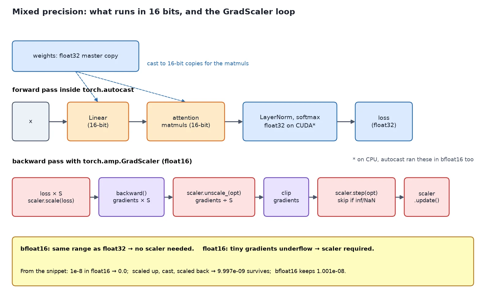

Mixed precision: what, why, how

What it is: running most of the maths in 16-bit floats.

Why it works: 16-bit numbers halve memory traffic, and GPU tensor cores multiply them much faster. Autocast keeps sensitive ops in float32 (on CUDA), and the weights stay float32.

How it works: wrap the forward pass and loss in torch.autocast(device, dtype=torch.bfloat16). For float16, also use torch.amp.GradScaler: scaler.scale(loss).backward(), scaler.unscale_(opt), clip, scaler.step(opt), scaler.update().

Step 3/6: torch.compile: Turning Python into Fused Kernels

In this step: We compile TinyDiT with torch.compile, look at its three stages, and check that it captures the whole model in one graph.

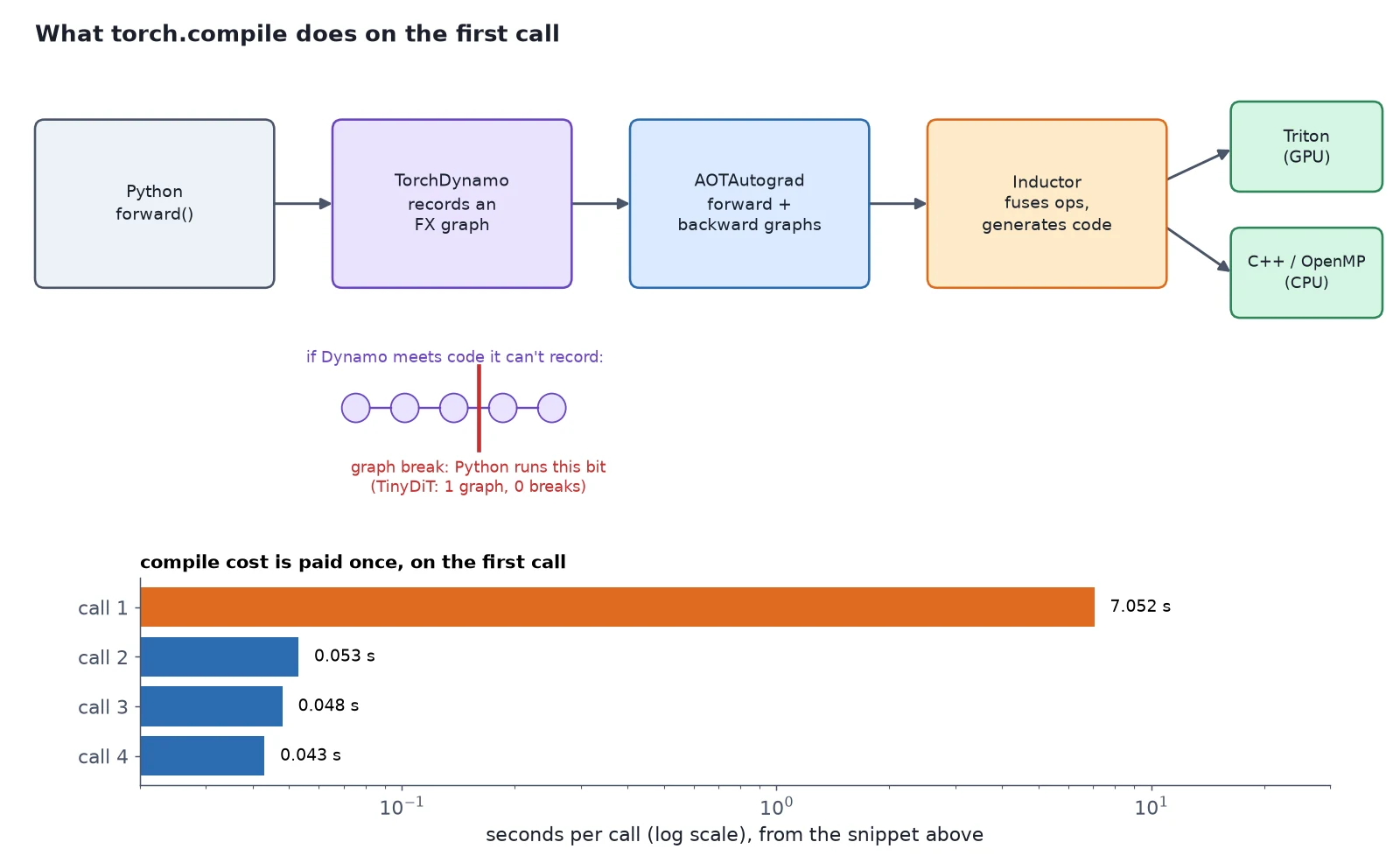
torch.compile(model) returns a version of the model that runs through a compiler. It has three stages:

1. TorchDynamo watches your Python forward run and records the tensor operations into a graph. If it meets something it can’t record, it splits the graph there (a graph break) and falls back to normal Python for that bit.
2. AOTAutograd builds the backward graph ahead of time, so training gets compiled too.
3. Inductor (the default backend) fuses many small operations into a few bigger kernels and generates code for them: Triton on NVIDIA GPUs, C++ with OpenMP on CPUs.

import time
import torch
from tinydit import TinyDiTConfig
from tinydit.model import TinyDiT

torch.manual_seed(0)
model = TinyDiT(TinyDiTConfig(dim=128, depth=4), use_sdpa=True).eval()
x, t = torch.randn(64, 3, 32, 32), torch.rand(64)

explanation = torch._dynamo.explain(model)(x, t)
print("graphs:", explanation.graph_count, "| graph breaks:", explanation.graph_break_count)

compiled = torch.compile(model)                         # nothing happens yet...
with torch.no_grad():
    for i in range(4):
        t0 = time.perf_counter()
        out = compiled(x, t)                            # ...the first call traces and compiles
        print(f"call {i + 1}: {time.perf_counter() - t0:.3f} s")
    print("matches eager:", torch.allclose(out, model(x, t), atol=1e-4))

import time
import torch
from tinydit import TinyDiTConfig
from tinydit.model import TinyDiT

torch.manual_seed(0)
model = TinyDiT(TinyDiTConfig(dim=128, depth=4), use_sdpa=True).eval()
x, t = torch.randn(64, 3, 32, 32), torch.rand(64)

explanation = torch._dynamo.explain(model)(x, t)
print("graphs:", explanation.graph_count, "| graph breaks:", explanation.graph_break_count)

compiled = torch.compile(model)                         # nothing happens yet...
with torch.no_grad():
    for i in range(4):
        t0 = time.perf_counter()
        out = compiled(x, t)                            # ...the first call traces and compiles
        print(f"call {i + 1}: {time.perf_counter() - t0:.3f} s")
    print("matches eager:", torch.allclose(out, model(x, t), atol=1e-4))

graphs: 1 | graph breaks: 0
call 1: 7.052 s
call 2: 0.053 s
call 3: 0.048 s
call 4: 0.043 s
matches eager: True

TinyDiT compiles into a single graph with no graph breaks, so the whole forward pass is captured. The first call took 7 seconds because that’s when compilation happens. After that, calls take milliseconds, and the output matches the uncompiled model.

torch.compile: what, why, how

What it is: a way to make a model run faster without rewriting it.

Why it works: TorchDynamo captures the forward pass as a graph, AOTAutograd adds the backward pass, and Inductor fuses small ops into fewer, bigger kernels.

How it works: net = torch.compile(model), then call net instead of model. The first call compiles (7 to 10 seconds here), later calls reuse the compiled code. Check for graph breaks with torch._dynamo.explain(model)(x, t).

Step 4/6: FastTrainer: Three Switches, Same Trainer

In this step: We add mixed precision and torch.compile to the post-5 Trainer as two switches, keeping a plain debug mode.

The constructor adds the two options. self.model stays the plain module (so checkpoints keep clean parameter names) and self.net is what we call, compiled or not:

"""FastTrainer (post 10): the post-5 Trainer plus mixed precision and torch.compile.

Nothing else changes: same loss_fn(model, batch), same fit / evaluate / save / load.
  amp_dtype=None            full float32 (the debug-friendly default)
  amp_dtype=torch.bfloat16  autocast to bfloat16 (CPU or recent GPUs; no scaler needed)
  amp_dtype=torch.float16   autocast to float16 + GradScaler (classic CUDA AMP)
  compile=True              run the forward/backward through torch.compile (Inductor)
"""
import torch
from torch import nn

from .trainer import Trainer, move_to


class FastTrainer(Trainer):
    def __init__(self, model: nn.Module, loss_fn, *, amp_dtype: torch.dtype | None = None,
                 compile: bool = False, **kwargs):
        super().__init__(model, loss_fn, **kwargs)
        self.amp_dtype = amp_dtype
        # GradScaler only matters for float16, whose small range can underflow gradients to zero.
        self.scaler = torch.amp.GradScaler(self.device.type, enabled=amp_dtype == torch.float16)
        # self.model stays the plain module (clean state_dict keys); self.net is what we call.
        self.net = torch.compile(self.model) if compile else self.model

"""FastTrainer (post 10): the post-5 Trainer plus mixed precision and torch.compile.

Nothing else changes: same loss_fn(model, batch), same fit / evaluate / save / load.
  amp_dtype=None            full float32 (the debug-friendly default)
  amp_dtype=torch.bfloat16  autocast to bfloat16 (CPU or recent GPUs; no scaler needed)
  amp_dtype=torch.float16   autocast to float16 + GradScaler (classic CUDA AMP)
  compile=True              run the forward/backward through torch.compile (Inductor)
"""
import torch
from torch import nn

from .trainer import Trainer, move_to


class FastTrainer(Trainer):
    def __init__(self, model: nn.Module, loss_fn, *, amp_dtype: torch.dtype | None = None,
                 compile: bool = False, **kwargs):
        super().__init__(model, loss_fn, **kwargs)
        self.amp_dtype = amp_dtype
        # GradScaler only matters for float16, whose small range can underflow gradients to zero.
        self.scaler = torch.amp.GradScaler(self.device.type, enabled=amp_dtype == torch.float16)
        # self.model stays the plain module (clean state_dict keys); self.net is what we call.
        self.net = torch.compile(self.model) if compile else self.model

train_step wraps the forward pass in autocast and routes the backward pass through the GradScaler:

    def train_step(self, batch) -> float:
        self.model.train()
        batch = move_to(batch, self.device)
        self.optimizer.zero_grad(set_to_none=True)
        with torch.autocast(self.device.type, dtype=self.amp_dtype or torch.float32,
                            enabled=self.amp_dtype is not None):
            loss = self.loss_fn(self.net, batch)          # forward runs in low precision where safe
        self.scaler.scale(loss).backward()                # backward outside autocast
        if self.max_grad_norm is not None:
            self.scaler.unscale_(self.optimizer)          # clip the real gradients, not scaled ones
            nn.utils.clip_grad_norm_(self.model.parameters(), self.max_grad_norm)
        self.scaler.step(self.optimizer)                  # skips the step if fp16 grads overflowed
        self.scaler.update()
        self.step += 1
        return loss.item()

    def train_step(self, batch) -> float:
        self.model.train()
        batch = move_to(batch, self.device)
        self.optimizer.zero_grad(set_to_none=True)
        with torch.autocast(self.device.type, dtype=self.amp_dtype or torch.float32,
                            enabled=self.amp_dtype is not None):
            loss = self.loss_fn(self.net, batch)          # forward runs in low precision where safe
        self.scaler.scale(loss).backward()                # backward outside autocast
        if self.max_grad_norm is not None:
            self.scaler.unscale_(self.optimizer)          # clip the real gradients, not scaled ones
            nn.utils.clip_grad_norm_(self.model.parameters(), self.max_grad_norm)
        self.scaler.step(self.optimizer)                  # skips the step if fp16 grads overflowed
        self.scaler.update()
        self.step += 1
        return loss.item()

With amp_dtype=None and compile=False, it does exactly what the post-5 Trainer does.

Step 5/6: The Benchmark: What Actually Got Faster?

In this step: We time five setups on full training steps and explain honestly why only SDPA helped on a CPU.

Now the honest test. Same 20 CIFAR-10 batches, same seed, five setups, timed on full training steps (forward, backward and AdamW update).

The five setups:

import time
import torch
from tinydit import TinyDiTConfig
from tinydit.data import CachedCIFAR10, make_loader
from tinydit.fast import FastTrainer
from tinydit.flow import flow_matching_loss
from tinydit.model import TinyDiT

cfg = TinyDiTConfig(dim=128, depth=4, num_heads=4)
loader = make_loader(CachedCIFAR10("data", train=True), batch_size=128, num_workers=0)
batches = [b for _, b in zip(range(20), loader)]               # same 20 batches for every setup

setups = [("post 9: eager, manual attention, fp32", dict(sdpa=False)),
          ("+ SDPA", dict(sdpa=True)),
          ("+ SDPA + bf16 autocast", dict(sdpa=True, amp_dtype=torch.bfloat16)),
          ("+ SDPA + torch.compile", dict(sdpa=True, compile=True)),
          ("+ SDPA + compile + bf16", dict(sdpa=True, compile=True, amp_dtype=torch.bfloat16))]

import time
import torch
from tinydit import TinyDiTConfig
from tinydit.data import CachedCIFAR10, make_loader
from tinydit.fast import FastTrainer
from tinydit.flow import flow_matching_loss
from tinydit.model import TinyDiT

cfg = TinyDiTConfig(dim=128, depth=4, num_heads=4)
loader = make_loader(CachedCIFAR10("data", train=True), batch_size=128, num_workers=0)
batches = [b for _, b in zip(range(20), loader)]               # same 20 batches for every setup

setups = [("post 9: eager, manual attention, fp32", dict(sdpa=False)),
          ("+ SDPA", dict(sdpa=True)),
          ("+ SDPA + bf16 autocast", dict(sdpa=True, amp_dtype=torch.bfloat16)),
          ("+ SDPA + torch.compile", dict(sdpa=True, compile=True)),
          ("+ SDPA + compile + bf16", dict(sdpa=True, compile=True, amp_dtype=torch.bfloat16))]

Each setup times the first step (which includes compiling), warms up, then times 45 steps:

for name, opts in setups:
    torch.manual_seed(0)
    model = TinyDiT(cfg, use_sdpa=opts.pop("sdpa"))
    trainer = FastTrainer(model, flow_matching_loss, lr=3e-4, **opts)
    t0 = time.perf_counter()
    trainer.train_step(batches[0])                             # first step (includes compiling)
    first = time.perf_counter() - t0
    for b in batches[1:5]:                                     # warm-up (compile can need a 2nd pass)
        trainer.train_step(b)
    t0 = time.perf_counter()
    for _ in range(3):
        for b in batches[5:]:
            loss = trainer.train_step(b)
    per_step = (time.perf_counter() - t0) / 45 * 1000
    print(f"{name:40s} first step {first:6.1f} s | {per_step:6.1f} ms/step | loss {loss:.3f}")

for name, opts in setups:
    torch.manual_seed(0)
    model = TinyDiT(cfg, use_sdpa=opts.pop("sdpa"))
    trainer = FastTrainer(model, flow_matching_loss, lr=3e-4, **opts)
    t0 = time.perf_counter()
    trainer.train_step(batches[0])                             # first step (includes compiling)
    first = time.perf_counter() - t0
    for b in batches[1:5]:                                     # warm-up (compile can need a 2nd pass)
        trainer.train_step(b)
    t0 = time.perf_counter()
    for _ in range(3):
        for b in batches[5:]:
            loss = trainer.train_step(b)
    per_step = (time.perf_counter() - t0) / 45 * 1000
    print(f"{name:40s} first step {first:6.1f} s | {per_step:6.1f} ms/step | loss {loss:.3f}")

post 9: eager, manual attention, fp32    first step    0.2 s |   75.7 ms/step | loss 0.558
+ SDPA                                   first step    0.1 s |   73.2 ms/step | loss 0.558
+ SDPA + bf16 autocast                   first step    0.1 s |   83.5 ms/step | loss 0.558
+ SDPA + torch.compile                   first step    8.3 s |  162.2 ms/step | loss 0.558
+ SDPA + compile + bf16                  first step    9.9 s |  165.0 ms/step | loss 0.559

All five setups give the same loss, so none of them changed the maths in a way that matters. But on this CPU only SDPA helped, and only by 3% end to end.

Why so little, when attention alone got 4.5× faster? Because with just 64 tokens, attention is a small part of TinyDiT’s work. Most of the time goes into the Linear layers of the FFNs and adaLN.

Why bfloat16 and compile were slower here

bfloat16 and torch.compile made training slower here, and that’s worth understanding rather than hiding:

• bfloat16 on a CPU saves little. The conversions to and from bfloat16 cost time, and a CPU doesn’t have the tensor cores that make 16-bit matmuls so fast on a GPU.
• torch.compile on a tiny CPU model has little to win. The big matmuls already call optimised libraries, and the fusions Inductor adds are small at this size. On my test machine the generated CPU code was also clearly slower than PyTorch’s own kernels.

On a GPU the picture is different, for the same reasons in reverse: tensor cores make bf16 matmuls several times faster than float32, and fusing many small kernels saves a lot of GPU launch overhead and memory traffic. That’s where PyTorch’s published compile speed-ups come from.

I haven’t measured it for TinyDiT on a GPU, so I won’t quote a number. Run 04_benchmark.py on your GPU and you’ll have your own.

Step 6/6: One Command per Experiment

In this step: We set up the single training script every Expert post uses, so all comparisons run with the same settings and scores.

The Expert posts compare many versions of TinyDiT. To keep those comparisons fair, every run goes through one script, code/train.py.

It builds the model from config flags, trains with FastTrainer, and writes a metrics.json with the loss curve, the held-out velocity MSE and probe-FD from post 9, the speed, and a sample grid:

# One experiment = one command. Every Expert post (11-14) runs its before/after this way.
cd code
python train.py --out runs/baseline --steps 4000 --set dim=128 --set depth=4      # CPU size
python train.py --out runs/gpu --steps 20000 --amp bf16 --compile                # on a GPU (defaults: dim 256, depth 6)
python train.py --out runs/debug --steps 50                                     # quick check, eager fp32
# each run writes runs/<name>/metrics.json (loss curve, velocity MSE, probe-FD, speed) and samples.png

# One experiment = one command. Every Expert post (11-14) runs its before/after this way.
cd code
python train.py --out runs/baseline --steps 4000 --set dim=128 --set depth=4      # CPU size
python train.py --out runs/gpu --steps 20000 --amp bf16 --compile                # on a GPU (defaults: dim 256, depth 6)
python train.py --out runs/debug --steps 50                                     # quick check, eager fp32
# each run writes runs/<name>/metrics.json (loss curve, velocity MSE, probe-FD, speed) and samples.png

Recap

• torch.compile, AMP and SDPA are each a one-line switch in our FastTrainer, and none of them changed the loss.
• SDPA made attention 4.5× faster and we keep it on everywhere.
• On an 8-core CPU, end-to-end training was only 3% faster with SDPA, about 10% slower with bfloat16 and about 2× slower with torch.compile (plus 8 seconds of compiling). Tiny CPU models are exactly the case where compile doesn’t pay.
• On a GPU, turn on bf16 and compile. That’s where they shine, but I didn’t measure TinyDiT on a GPU, so there are no GPU numbers here.
• Every Expert experiment from now on is one train.py command with the same settings and the same scores.

Next up: The Expert posts begin. In RMSNorm, QK-Norm, SwiGLU, and 2D RoPE in a Tiny DiT we upgrade the transformer block itself with RMSNorm, QK-norm, SwiGLU and 2D RoPE, and measure each change on its own.

← Previous: Post 9: Build a Tiny Diffusion Transformer in PyTorch (DiT from Scratch)
Next → Post 11: RMSNorm, QK-Norm, SwiGLU, and 2D RoPE in a Tiny DiT