Patch Embeddings in PyTorch: How a Transformer Reads an Image
Where you are: Post 7 of 14 in PyTorch Tutorial 2026 · about 12 min read
What you’ll build: tinydit/patches.py: patchify and unpatchify, a PatchEmbed layer, a learned 2D position embedding and a PatchHead. Together they make TinyDiT’s “image in, image out” skeleton, trained on real CIFAR-10.
You’ll need: Post 2 (reshape and permute), Post 5 (Trainer) and Post 6 (TransformerBlock).
In this post:
- Introduction
- Step 1/6: Why Cut Images into Patches?
- Step 2/6: patchify and unpatchify
- Step 3/6: PyTorch Patch Embedding: From 48 Numbers to a Token
- Step 4/6: Position Embeddings: Telling Patches Where They Are
- Step 5/6: PatchHead: The Output Side
- Step 6/6: Train the Image-In, Image-Out Transformer
- Recap
Series: PyTorch Tutorial 2026 (14 posts)
- Post 1: PyTorch Tutorial 2026: From Tensors to Tiny Diffusion
- Post 2: PyTorch Tensors Explained: Shapes, Broadcasting, and Images as Arrays
- Post 3: PyTorch Autograd: How backward() Builds Gradients
- Post 4: PyTorch DataLoader Explained: Datasets, Batches, and Image Folders
- Post 5: PyTorch nn.Module and the Training Loop: Layers, Loss, and Checkpoints
- Post 6: Attention and the Transformer Block in PyTorch
- Post 7: Patch Embeddings in PyTorch: How a Transformer Reads an Image (you are here)
- Post 8: Flow Matching in PyTorch: Train a Model to Follow a Straight Line
- Post 9: Build a Tiny Diffusion Transformer in PyTorch (DiT from Scratch)
- Post 10: torch.compile, Mixed Precision, and SDPA: Speed Up TinyDiT
- Post 11: RMSNorm, QK-Norm, SwiGLU, and 2D RoPE in a Tiny DiT
- Post 12: adaLN-Zero and Classifier-Free Guidance in PyTorch
- Post 13: MMDiT Joint Attention in PyTorch: Two Streams, One Generator
- Post 14: Train and Sample Like 2026: Logit-Normal Steps, EMA, and Few-Step Flow
Introduction
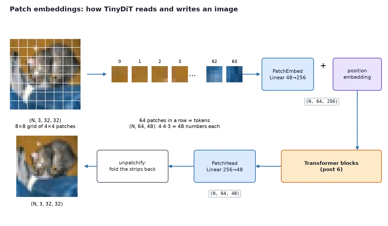
A transformer reads a sequence of tokens. An image is a grid of pixels. Patch embeddings are the bridge: cut the image into small squares, flatten each square, and turn it into a token with one Linear layer.
In this PyTorch patch embedding tutorial we write patchify and unpatchify from scratch for 32×32 CIFAR-10 images (patch size 4, so 64 tokens), build a PatchEmbed layer, add a learned 2D position embedding so the model knows where each patch sits, and fold tokens back into an image with a PatchHead. These are TinyDiT’s input and output: the first and last layers of the generator.
In Attention and the Transformer Block in PyTorch we built the TransformerBlock, which maps (N, L, D) to (N, L, D). Today we produce that (N, L, D) from images, and turn it back into images afterwards. By the end, we’ll have a complete “image in, image out” transformer and train it on real CIFAR-10 data.
Step 1/6: Why Cut Images into Patches?
In this step: We see why a transformer reads an image as 64 patch tokens instead of 1,024 pixels, and fix our sizes in one config file.
We could treat every pixel as a token: 32 × 32 = 1,024 tokens per image. Attention compares every token with every other token, so that’s about a million comparisons per head per layer. It’s also wasteful: a single pixel carries very little meaning on its own.
Cutting the image into 4×4 patches gives an 8×8 grid, so 64 tokens, each holding 4 × 4 × 3 = 48 numbers. That means 256× fewer attention pairs, and each token is a meaningful little piece of the picture (an edge, a bit of fur, a patch of sky).
\begin{gathered} \underbrace{L}_{\text{tokens}} = \frac{H}{p} \cdot \frac{W}{p} = \frac{32}{4} \cdot \frac{32}{4} = 64 \\ \underbrace{p \cdot p \cdot C}_{\text{numbers per patch}} = 4 \cdot 4 \cdot 3 = 48 \\ \underbrace{L^{2}}_{\text{attention pairs}} = 4{,}096 \;\text{ vs }\; 1{,}024^{2} \approx 10^{6} \end{gathered}This is exactly the input of the Vision Transformer (Dosovitskiy et al., An Image is Worth 16×16 Words, 2020). DiT (Peebles and Xie, 2023) reads its input the same way, and so does every DiT-style generator since, including SD3 and FLUX (which patchify a compressed latent instead of raw pixels).
Note: The patch size is the main knob that trades detail against compute: DiT found that smaller patches (more tokens) give clearly better images at a higher cost.
Our sizes live in one place, tinydit/config.py, so every later post uses the same numbers:
"""Default sizes for TinyDiT. Later posts may ADD fields; do not rename these."""
from dataclasses import dataclass


@dataclass
class TinyDiTConfig:
    img_size: int = 32        # CIFAR-10 is 32x32
    in_channels: int = 3      # RGB
    patch_size: int = 4       # 32 / 4 = 8 -> 8x8 grid = 64 tokens
    dim: int = 256            # token width D
    depth: int = 6            # number of transformer blocks
    num_heads: int = 4        # head_dim = 256 / 4 = 64
    mlp_ratio: float = 4.0    # FFN hidden = 4 * D
    num_classes: int = 10     # CIFAR-10 labels (used from post 12)

    @property
    def grid_size(self) -> int:
        return self.img_size // self.patch_size

    @property
    def num_patches(self) -> int:
        return self.grid_size ** 2

    @property
    def patch_dim(self) -> int:
return self.patch_size * self.patch_size * self.in_channelsWhat you just built: tinydit/config.py with TinyDiT’s sizes: 32×32 images, patch size 4, 64 tokens of 48 numbers, D = 256.
Step 2/6: patchify and unpatchify
In this step: We cut images into patch tokens with only reshape and permute, and fold tokens back into images exactly.
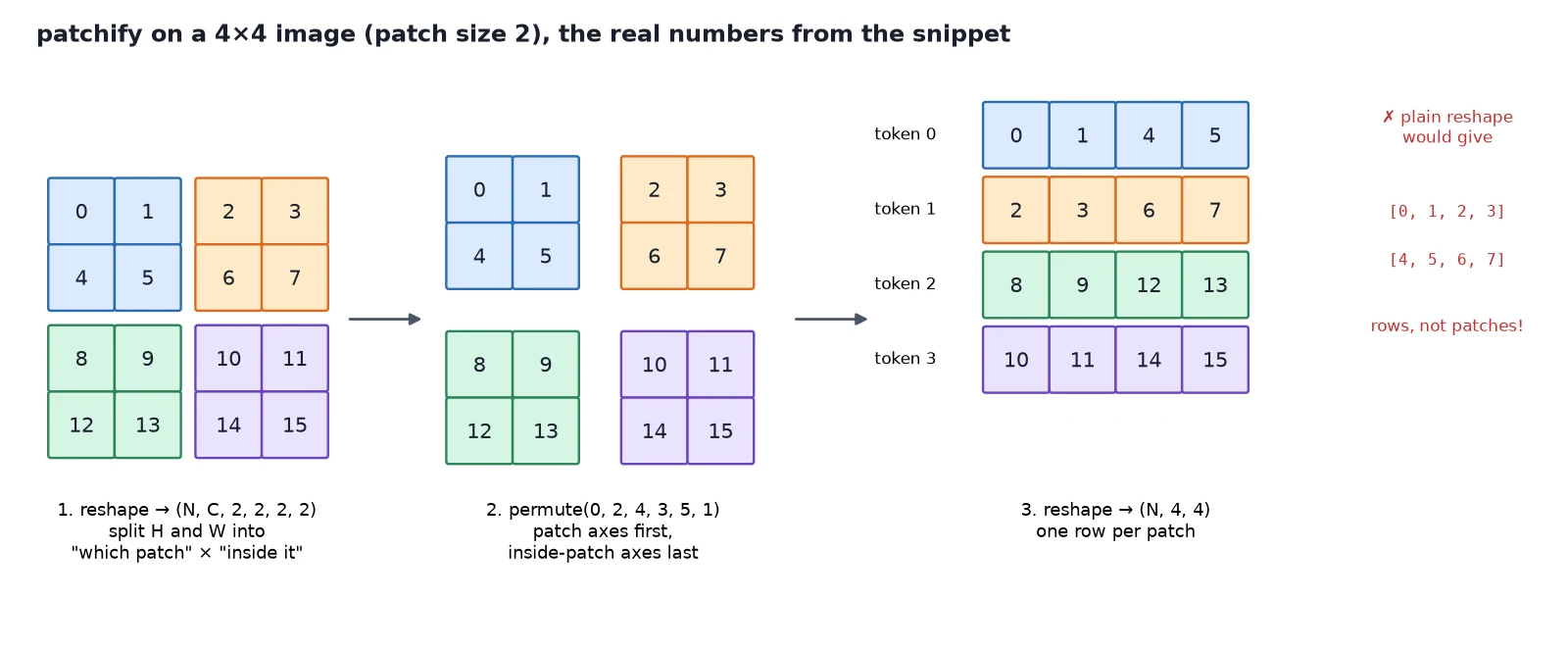
The trick is to do it with reshape and permute only, no loops. Let’s watch it on a tiny 4×4 one-channel “image” with patch size 2, so we can follow every number:
import torch
from tinydit.patches import patchify, unpatchify

# One 1-channel 4x4 "image" with easy-to-follow numbers, patch size 2 -> a 2x2 grid of patches.
x = torch.arange(16.0).reshape(1, 1, 4, 4)
print(x[0, 0])

p = 2
step1 = x.reshape(1, 1, 2, p, 2, p)       # (N, C, grid_h, p, grid_w, p): split H and W
step2 = step1.permute(0, 2, 4, 3, 5, 1)   # (N, grid_h, grid_w, p, p, C): patch axes together
tokens = step2.reshape(1, 4, p * p * 1)   # (N, L, p*p*C): one row per patch
print(tokens[0])
print("same as patchify():", torch.equal(tokens, patchify(x, p)))
print("round trip exact: ", torch.equal(unpatchify(tokens, p, 1, 4, 4), x))tensor([[ 0., 1., 2., 3.],
[ 4., 5., 6., 7.],
[ 8., 9., 10., 11.],
[12., 13., 14., 15.]])
tensor([[ 0., 1., 4., 5.],
[ 2., 3., 6., 7.],
[ 8., 9., 12., 13.],
[10., 11., 14., 15.]])
same as patchify(): True
round trip exact: TrueRow 0 of the output is the top-left 2×2 patch [0, 1, 4, 5]. Row 1 is the top-right patch [2, 3, 6, 7], and so on. Here’s what each step did:
reshape(N, C, H/p, p, W/p, p): split the height axis into “which patch row” × “row inside the patch”, and the same for width. No data moves; we just reinterpret the axes.permute(0, 2, 4, 3, 5, 1): reorder to(N, patch_row, patch_col, inner_row, inner_col, C). This puts the two “which patch” axes first and everything inside a patch last. This is the step a plainreshapecan’t do.reshape(N, L, p·p·C): merge the patch-grid axes into one sequence axis, and the inside-a-patch axes into one feature axis.
In tinydit/patches.py, patchify is exactly those three steps:
"""Images <-> tokens (post 7). TinyDiT's input and output heads.

Patch flattening order is (p_row, p_col, channel) everywhere in the series.
"""
import torch
from torch import nn


def patchify(x: torch.Tensor, patch_size: int) -> torch.Tensor:
    """(N, C, H, W) -> (N, L, p*p*C) with L = (H/p) * (W/p), row-major over the patch grid."""
    n, c, h, w = x.shape
    p = patch_size
    assert h % p == 0 and w % p == 0, "H and W must be divisible by patch_size"
    gh, gw = h // p, w // p
    x = x.reshape(n, c, gh, p, gw, p)          # split H into (gh, p) and W into (gw, p)
    x = x.permute(0, 2, 4, 3, 5, 1)            # (N, gh, gw, p, p, C)
return x.reshape(n, gh * gw, p * p * c)Here’s the same thing at TinyDiT size, plus two sanity checks:
import torch
from tinydit import TinyDiTConfig
from tinydit.patches import patchify, unpatchify

cfg = TinyDiTConfig()
print(cfg)
print("grid:", cfg.grid_size, "x", cfg.grid_size, "| tokens:", cfg.num_patches, "| numbers per patch:", cfg.patch_dim)

x = torch.rand(8, 3, 32, 32) * 2 - 1          # a batch of 8 images in [-1, 1]
t = patchify(x, cfg.patch_size)
print("patchify:  ", tuple(x.shape), "->", tuple(t.shape))
back = unpatchify(t, cfg.patch_size, 3, 32, 32)
print("unpatchify:", tuple(t.shape), "->", tuple(back.shape), "| exact:", torch.equal(back, x))

# Token 9 = grid row 1, column 1 = pixels [4:8, 4:8]
print("token 9 is the patch at rows 4-7, cols 4-7:",
      torch.equal(t[0, 9], x[0, :, 4:8, 4:8].permute(1, 2, 0).reshape(-1)))

wrong = x.reshape(8, 64, 48)                  # same shape, wrong meaning!
print("plain reshape gives real patches?", torch.equal(wrong, t))TinyDiTConfig(img_size=32, in_channels=3, patch_size=4, dim=256, depth=6, num_heads=4, mlp_ratio=4.0, num_classes=10)
grid: 8 x 8 | tokens: 64 | numbers per patch: 48
patchify: (8, 3, 32, 32) -> (8, 64, 48)
unpatchify: (8, 64, 48) -> (8, 3, 32, 32) | exact: True
token 9 is the patch at rows 4-7, cols 4-7: True
plain reshape gives real patches? FalseToken 9 is grid row 1, column 1 (since 9 = 1 \cdot 8 + 1), which is pixels 4–7 in both directions. The tokens are numbered row-major, left to right, then top to bottom, like reading a page.
Watch out: A plain reshape(8, 64, 48) gives the right shape but the wrong content, the same trap we saw with HWC versus CHW in post 2.
And here’s what the transformer actually “reads” for a real CIFAR-10 test image:
import torch
from tinydit.data import get_cifar10
from tinydit.images import save_image, save_grid
from tinydit.patches import patchify

x, label = get_cifar10("data", train=False)[0]          # one test image, (3, 32, 32)
tokens = patchify(x.unsqueeze(0), 4)                     # (1, 64, 48)
print("image", tuple(x.shape), "-> tokens", tuple(tokens.shape))

# Turn each token back into a little 4x4 picture, to see what the transformer "reads".
patches = tokens[0].reshape(64, 4, 4, 3).permute(0, 3, 1, 2)   # (64, 3, 4, 4)
save_image(x, "image.png")
save_grid(patches, "patches_as_sequence.png", nrow=64)          # one long row = the token sequence
save_grid(patches, "patches_as_grid.png", nrow=8)               # same tokens, folded 8 x 8
print("saved image.png, patches_as_sequence.png, patches_as_grid.png")image (3, 32, 32) -> tokens (1, 64, 48)
saved image.png, patches_as_sequence.png, patches_as_grid.png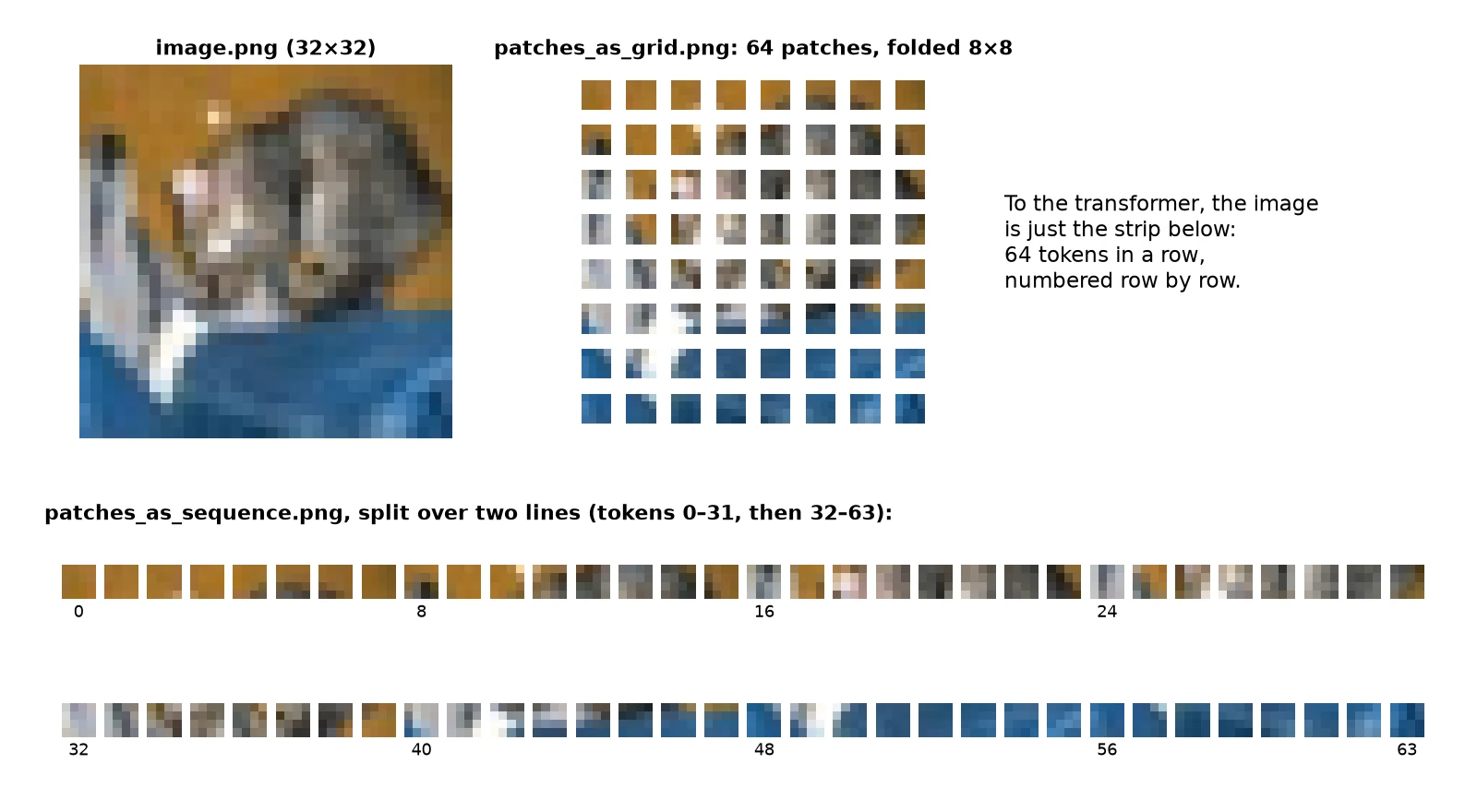
unpatchify: tokens back to an image
unpatchify runs the same three steps in reverse: split the sequence axis back into (patch_row, patch_col) and the feature axis into (inner_row, inner_col, C), permute back, and merge:
def unpatchify(tokens: torch.Tensor, patch_size: int, channels: int,
               height: int, width: int) -> torch.Tensor:
    """Exact inverse of patchify: (N, L, p*p*C) -> (N, C, H, W)."""
    n = tokens.shape[0]
    p = patch_size
    gh, gw = height // p, width // p
    x = tokens.reshape(n, gh, gw, p, p, channels)
    x = x.permute(0, 5, 1, 3, 2, 4)            # (N, C, gh, p, gw, p)
return x.reshape(n, channels, height, width)Because both directions only reshape and permute, the round trip is exact: torch.equal, not just “close”.
Why it works: Our generator has to output something image-shaped. From post 8 onward, TinyDiT predicts a velocity (which direction to move each pixel), and that velocity has the same (N, 3, 32, 32) shape as the image. The transformer produces tokens, and unpatchify turns them back into pixels.
What you just built: patchify and unpatchify: (N, 3, 32, 32) ↔ (N, 64, 48), row-major, with an exact round trip.
Step 3/6: PyTorch Patch Embedding: From 48 Numbers to a Token
In this step: We turn each 48-number patch into a 256-feature token with one shared Linear layer, and show it is the same layer as a strided convolution.
A flattened patch is 48 raw pixel values. The transformer works with D = 256 features per token. One nn.Linear(48, 256), shared by all 64 patches, makes the jump:
\begin{gathered} \underbrace{e_i}_{\text{token } i,\ (256)} = \underbrace{\operatorname{flatten}(\text{patch}_i)}_{(48)}\, \underbrace{W_E^{\top}}_{(48 \times 256)} + \underbrace{b_E}_{(256)} \\ i = 0, \dots, 63 \end{gathered}In code, PatchEmbed is patchify followed by that Linear:
class PatchEmbed(nn.Module):
    """Cut into patches, flatten, Linear. (N, C, H, W) -> (N, L, dim)."""

    def __init__(self, img_size: int = 32, patch_size: int = 4, in_channels: int = 3, dim: int = 256):
        super().__init__()
        self.patch_size = patch_size
        self.grid_size = img_size // patch_size
        self.num_patches = self.grid_size ** 2
        self.proj = nn.Linear(patch_size * patch_size * in_channels, dim)

    def forward(self, x: torch.Tensor) -> torch.Tensor:
return self.proj(patchify(x, self.patch_size))import torch
from torch import nn
from tinydit.patches import PatchEmbed
torch.manual_seed(0)
embed = PatchEmbed(img_size=32, patch_size=4, in_channels=3, dim=256)
x = torch.randn(2, 3, 32, 32)
tokens = embed(x)
print("PatchEmbed:", tuple(x.shape), "->", tuple(tokens.shape))
print("Linear weight:", tuple(embed.proj.weight.shape), "| params:", sum(p.numel() for p in embed.parameters()))
# The same layer written as a Conv2d with kernel = stride = patch size (how many ViT/DiT repos do it).
conv = nn.Conv2d(3, 256, kernel_size=4, stride=4)
with torch.no_grad():
# Linear expects (p_row, p_col, C) order; Conv2d stores (out, C, p_row, p_col).
conv.weight.copy_(embed.proj.weight.reshape(256, 4, 4, 3).permute(0, 3, 1, 2))
conv.bias.copy_(embed.proj.bias)
conv_tokens = conv(x).flatten(2).transpose(1, 2) # (N, 256, 8, 8) -> (N, 64, 256)
print("Conv2d version identical:", torch.allclose(tokens, conv_tokens, atol=1e-5))PatchEmbed: (2, 3, 32, 32) -> (2, 64, 256)
Linear weight: (256, 48) | params: 12544
Conv2d version identical: TrueYou’ll often see patch embeddings written as nn.Conv2d(3, D, kernel_size=p, stride=p), a convolution that jumps a whole patch at a time. As the output shows, it’s the same layer: each output position is a weighted sum of one 4×4×3 patch. The only difference is how the weights are stored in memory.
Note: We use the Linear form because it makes “flatten a patch, then Linear” visible, and because patchify and unpatchify are needed anyway for the output side.
PatchEmbed: what, why, how
What it is: the layer that turns a picture into a sequence of tokens: (N, 3, 32, 32) → (N, 64, 256).
Why it works: transformers run on sequences, so the image has to become one. Small patches keep nearby pixels together, since the pixels inside a 4×4 square are strongly related, and they cut the sequence length from 1,024 to 64, which makes attention 256× cheaper. A shared Linear means every patch is embedded the same way wherever it sits, and position is added separately.
How it works: cut with reshape, reorder with permute, flatten each patch to 48 numbers (patchify), then nn.Linear(48, 256). That’s equivalent to nn.Conv2d(3, 256, kernel_size=4, stride=4).
What you just built: PatchEmbed: (N, 3, 32, 32) → (N, 64, 256), checked against the equivalent strided Conv2d.
Step 4/6: Position Embeddings: Telling Patches Where They Are
In this step: We show that attention ignores token order, then fix it with a learned 2D position embedding.
Here’s a surprising fact about attention: it has no idea where tokens are. Shuffle the input tokens and a transformer block just shuffles its output the same way:
import torch
from tinydit.blocks import TransformerBlock

torch.manual_seed(0)
block = TransformerBlock(256, 4).eval()
tokens = torch.randn(1, 64, 256)

perm = torch.randperm(64)                 # shuffle the patches
out = block(tokens)
out_shuffled = block(tokens[:, perm])

# Shuffling the input just shuffles the output the same way:
print("block(shuffle(x)) == shuffle(block(x)):", torch.allclose(out_shuffled, out[:, perm], atol=1e-5))block(shuffle(x)) == shuffle(block(x)): TrueTo attention, a picture with the sky at the top and one with the sky at the bottom are the same bag of patches. That’s useless for generating images, so we add a position vector to each token. Each grid slot gets its own vector, and the model learns what those vectors should be.
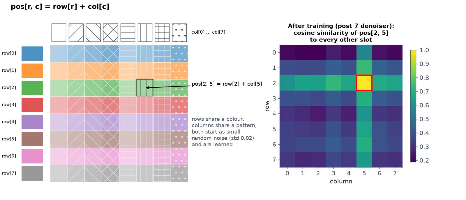
We use a 2D-aware learned table. Instead of 64 independent vectors, we learn one vector per row and one per column, and the embedding for the slot at row r, column c is their sum:
\begin{gathered} \underbrace{\text{pos}[r, c]}_{\text{slot } (r, c),\ (256)} = \underbrace{\text{row}[r]}_{\text{learned, } 8 \times 256} + \underbrace{\text{col}[c]}_{\text{learned, } 8 \times 256} \\ \text{token}_{r \cdot 8 + c} \;\leftarrow\; e_{r \cdot 8 + c} + \text{pos}[r, c] \end{gathered}This bakes in the fact that the grid has two axes: all patches in row 2 share row[2], so the model gets “same height” for free. It also uses 4,096 numbers instead of 16,384.
Under the hood it’s just broadcasting from post 2: row[:, None, :] + col[None, :, :] turns (8, 1, 256) + (1, 8, 256) into (8, 8, 256):
class PosEmbed2D(nn.Module):
    """Learned 2D-aware position embedding: pos[r, c] = row[r] + col[c].

    Adds (1, L, dim) to tokens (N, L, dim). L = grid_size ** 2, row-major.
    """

    def __init__(self, grid_size: int = 8, dim: int = 256):
        super().__init__()
        self.grid_size = grid_size
        self.row = nn.Parameter(torch.randn(grid_size, dim) * 0.02)
        self.col = nn.Parameter(torch.randn(grid_size, dim) * 0.02)

    def table(self) -> torch.Tensor:
        """(1, L, dim) table, one vector per grid slot."""
        g = self.grid_size
        pos = self.row[:, None, :] + self.col[None, :, :]   # (g, g, dim) via broadcasting
        return pos.reshape(1, g * g, -1)

    def forward(self, tokens: torch.Tensor) -> torch.Tensor:
return tokens + self.table()import torch
from tinydit.blocks import TransformerBlock
from tinydit.patches import PosEmbed2D
torch.manual_seed(0)
pos = PosEmbed2D(grid_size=8, dim=256)
print("row table:", tuple(pos.row.shape), "| col table:", tuple(pos.col.shape))
print("full table:", tuple(pos.table().shape), "| learned numbers:", sum(p.numel() for p in pos.parameters()))
table = pos.table()[0] # (64, 256)
r, c = 2, 5
print("slot (2,5) = row[2] + col[5]:", torch.allclose(table[r * 8 + c], pos.row[r] + pos.col[c]))
block = TransformerBlock(256, 4).eval()
tokens = torch.randn(1, 64, 256)
perm = torch.randperm(64)
out = block(pos(tokens))
out_shuffled = block(pos(tokens[:, perm]))
print("with positions, shuffling still commutes?", torch.allclose(out_shuffled, out[:, perm], atol=1e-5))row table: (8, 256) | col table: (8, 256)
full table: (1, 64, 256) | learned numbers: 4096
slot (2,5) = row[2] + col[5]: True
with positions, shuffling still commutes? FalseWith positions added, shuffling the patches changes the result. The model can now tell where everything is.
Note: DiT itself uses a fixed 2D sine-cosine table instead of a learned one. Both work at this size. We start with a learned table because it’s the simplest idea to see; in Expert post 11 we replace it with 2D RoPE, the rotary position scheme FLUX uses, which builds relative position directly into attention.
Position embedding (PosEmbed2D): what, why, how
What it is: a per-location signal added to every token, so the model knows which patch is where.
Why it works: attention treats its input as an unordered set, as we showed: shuffling in means shuffling out. Adding a different learned vector at each grid slot makes identical patches at different places look different to the model, and training teaches the vectors to encode “top”, “left”, “next to” and so on. Splitting it into row and column vectors gives the model the 2D structure of the grid up front.
How it works: two learned tables, row (8, 256) and col (8, 256), start as small random numbers. Broadcasting builds the (64, 256) table row[r] + col[c], which is added to the tokens right after PatchEmbed.
What you just built: PosEmbed2D: a learned 2D-aware position table that makes the model sensitive to where each patch sits.
Step 5/6: PatchHead: The Output Side
In this step: We mirror the input side with a PatchHead that turns tokens back into an image-shaped tensor, completing TinyDiT’s skeleton.
The output layer mirrors the input: a LayerNorm, a Linear from D = 256 back to 48 numbers per token, then unpatchify:
class PatchHead(nn.Module):
    """Tokens back to an image-shaped tensor: LayerNorm, Linear(dim -> p*p*C), unpatchify.

    (N, L, dim) -> (N, C, H, W). TinyDiT uses this to emit a velocity field (post 9
    swaps the LayerNorm for an adaLN-modulated one).
    """

    def __init__(self, img_size: int = 32, patch_size: int = 4, out_channels: int = 3, dim: int = 256):
        super().__init__()
        self.img_size, self.patch_size, self.out_channels = img_size, patch_size, out_channels
        self.norm = nn.LayerNorm(dim)
        self.proj = nn.Linear(dim, patch_size * patch_size * out_channels)

    def forward(self, tokens: torch.Tensor) -> torch.Tensor:
        x = self.proj(self.norm(tokens))
return unpatchify(x, self.patch_size, self.out_channels, self.img_size, self.img_size)Here’s the full skeleton, image in and image out:
import torch
from tinydit.patches import PatchEmbed, PosEmbed2D, PatchHead
from tinydit.blocks import TransformerBlock

torch.manual_seed(0)
embed, pos, head = PatchEmbed(), PosEmbed2D(), PatchHead()
blocks = torch.nn.Sequential(*[TransformerBlock(256, 4) for _ in range(2)])

x = torch.randn(4, 3, 32, 32)
t = embed(x);  print("PatchEmbed  ", tuple(x.shape), "->", tuple(t.shape))
t = pos(t);    print("PosEmbed2D  ", tuple(t.shape), "->", tuple(t.shape))
t = blocks(t); print("blocks x2   ", tuple(t.shape), "->", tuple(t.shape))
y = head(t);   print("PatchHead   ", tuple(t.shape), "->", tuple(y.shape))
print("head params:", sum(p.numel() for p in head.parameters()))PatchEmbed (4, 3, 32, 32) -> (4, 64, 256)
PosEmbed2D (4, 64, 256) -> (4, 64, 256)
blocks x2 (4, 64, 256) -> (4, 64, 256)
PatchHead (4, 64, 256) -> (4, 3, 32, 32)
head params: 12848| Stage | Shape |
|---|---|
| Input images | (N, 3, 32, 32) |
patchify | (N, 64, 48) |
PatchEmbed (Linear 48 → 256) | (N, 64, 256) |
+ PosEmbed2D | (N, 64, 256) |
TransformerBlock × depth | (N, 64, 256) |
PatchHead (LayerNorm, Linear 256 → 48) | (N, 64, 48) |
unpatchify | (N, 3, 32, 32) |
That’s TinyDiT’s skeleton. In post 9, the only structural addition is a timestep input that tells each block how noisy the picture is.
Unpatchify and PatchHead: what, why, how
What it is: the layer that turns tokens back into an image-shaped tensor: (N, 64, 256) → (N, 3, 32, 32).
Why it works: the flow-matching target in post 8 is an image-shaped velocity, one value per pixel and channel, so the model’s output must be a picture-shaped tensor, not a sequence.
How it works: PatchHead applies LayerNorm and nn.Linear(256, 48) to every token, then unpatchify reverses patchify‘s reshape and permute, exactly. In post 9 the LayerNorm gets a timestep-dependent scale and shift, like every block in DiT.
What you just built: PatchHead and the full skeleton: PatchEmbed → PosEmbed2D → TransformerBlocks → PatchHead, image in, image out.
Step 6/6: Train the Image-In, Image-Out Transformer
In this step: We train the skeleton as a denoiser on real CIFAR-10 and compare it with the patch-by-patch model from post 5.
Let’s give the skeleton the same job we gave the patch denoiser in post 5: clean up images with Gaussian noise of strength 0.5. The difference is that the post-5 model cleaned each 4×4 patch on its own, while this one can use attention to look at every other patch.
The model in examples/image_denoiser.py chains the four pieces:
"""Image in, image out: PatchEmbed -> PosEmbed2D -> TransformerBlocks -> PatchHead (post 7).

Same noisy-patch task as examples/patch_denoiser.py, but now every patch can
look at every other patch through attention. TinyDiT (post 9) is this skeleton
plus a timestep input.
"""
import torch
import torch.nn.functional as F
from torch import nn

from tinydit.blocks import TransformerBlock
from tinydit.patches import PatchEmbed, PatchHead, PosEmbed2D

NOISE = 0.5


class ImageDenoiser(nn.Module):
    def __init__(self, img_size=32, patch_size=4, channels=3, dim=128, depth=2, num_heads=4):
        super().__init__()
        self.embed = PatchEmbed(img_size, patch_size, channels, dim)
        self.pos = PosEmbed2D(img_size // patch_size, dim)
        self.blocks = nn.Sequential(*[TransformerBlock(dim, num_heads) for _ in range(depth)])
        self.head = PatchHead(img_size, patch_size, channels, dim)

    def forward(self, x: torch.Tensor) -> torch.Tensor:   # (N, 3, 32, 32) -> (N, 3, 32, 32)
return self.head(self.blocks(self.pos(self.embed(x))))The loss is the same noisy-image task, now on whole images:
def denoise_loss(model: nn.Module, batch) -> torch.Tensor:
    images, _labels = batch
    noisy = images + NOISE * torch.randn_like(images)
return F.mse_loss(model(noisy), images)Same data, same 300 CPU steps, same Trainer:
import torch
from tinydit import get_device
from tinydit.data import get_cifar10, make_loader
from tinydit.trainer import Trainer
from examples.image_denoiser import ImageDenoiser, denoise_loss

torch.manual_seed(0)
train_loader = make_loader(get_cifar10("data", train=True, limit=8192), batch_size=128, num_workers=2)
test_loader = make_loader(get_cifar10("data", train=False, limit=1024), batch_size=256,
                          shuffle=False, num_workers=0)

model = ImageDenoiser(dim=128, depth=2, num_heads=4)
print("params:", sum(p.numel() for p in model.parameters()))
trainer = Trainer(model, denoise_loss, device=get_device(), lr=1e-3)
trainer.fit(train_loader, max_steps=300, log_every=100, ckpt_path="checkpoints/image_denoiser.pt")
print("held-out loss:", round(trainer.evaluate(test_loader), 4))
print("post 5 PatchDenoiser (patches on their own) scored 0.0301; doing nothing scores 0.25")params: 411312
step 100 | loss 0.0486
step 200 | loss 0.0284
step 300 | loss 0.0270
held-out loss: 0.0268
post 5 PatchDenoiser (patches on their own) scored 0.0301; doing nothing scores 0.25The held-out error drops from 0.0301 to 0.0268, about 11% lower, from a model of similar size (411K vs 277K parameters) trained for the same number of steps.
Why it works: Being able to look at neighbouring patches helps: a patch of noisy sky is easier to clean when you can see the sky all around it. It’s a modest gain at this tiny scale, but it’s the first time our model has treated the picture as a whole.
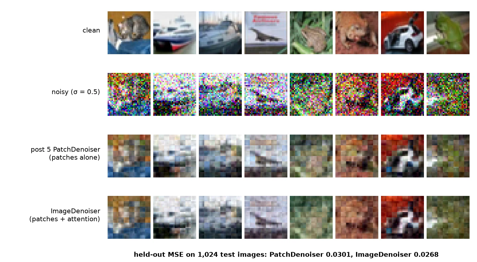
Note: This is still a denoiser, not a generator: it can clean a picture, but it can’t make one from nothing. Getting from “remove some noise” to “turn pure noise into a picture” is what flow matching does in the next post.
What you just built: An ImageDenoiser that beats the post-5 patch denoiser on held-out data (MSE 0.0268 vs 0.0301).
Recap
- PyTorch patch embedding =
patchify(reshape, permute, reshape) + onenn.Linear. For CIFAR with p = 4:(N, 3, 32, 32)→(N, 64, 48)→(N, 64, 256). unpatchifyis the exact inverse. Plainreshapegives the right shape but the wrong patches.- A Linear on flattened patches is the same layer as a strided
Conv2d. - Attention ignores order, so we add a learned 2D-aware position embedding, \text{pos}[r, c] = \text{row}[r] + \text{col}[c].
PatchEmbed → PosEmbed2D → TransformerBlocks → PatchHeadis TinyDiT’s skeleton. As a denoiser it beat the patch-by-patch model from post 5 (held-out MSE 0.0268 vs 0.0301).
Next up: In Flow Matching in PyTorch: Train a Model to Follow a Straight Line comes the idea that turns this skeleton into a generator: flow matching, where we train a model to follow a straight line from noise to data.
Series: PyTorch Tutorial 2026 (14 posts)
- Post 1: PyTorch Tutorial 2026: From Tensors to Tiny Diffusion
- Post 2: PyTorch Tensors Explained: Shapes, Broadcasting, and Images as Arrays
- Post 3: PyTorch Autograd: How backward() Builds Gradients
- Post 4: PyTorch DataLoader Explained: Datasets, Batches, and Image Folders
- Post 5: PyTorch nn.Module and the Training Loop: Layers, Loss, and Checkpoints
- Post 6: Attention and the Transformer Block in PyTorch
- Post 7: Patch Embeddings in PyTorch: How a Transformer Reads an Image (you are here)
- Post 8: Flow Matching in PyTorch: Train a Model to Follow a Straight Line
- Post 9: Build a Tiny Diffusion Transformer in PyTorch (DiT from Scratch)
- Post 10: torch.compile, Mixed Precision, and SDPA: Speed Up TinyDiT
- Post 11: RMSNorm, QK-Norm, SwiGLU, and 2D RoPE in a Tiny DiT
- Post 12: adaLN-Zero and Classifier-Free Guidance in PyTorch
- Post 13: MMDiT Joint Attention in PyTorch: Two Streams, One Generator
- Post 14: Train and Sample Like 2026: Logit-Normal Steps, EMA, and Few-Step Flow
← Previous: Post 6: Attention and the Transformer Block in PyTorch
Next → Post 8: Flow Matching in PyTorch: Train a Model to Follow a Straight Line