PyTorch Autograd: How backward() Builds Gradients
Where you are: Post 3 of 14 in PyTorch Tutorial 2026 · about 9 min read
What you’ll build: A clear model of how loss.backward() computes gradients, why every training loop calls zero_grad(), and examples/fit_line.py, a line fit with nothing but tensors and autograd.
You’ll need: Post 2 (tensors: shape, dtype, device).
In this post:
- Introduction
- Step 1/6: Why We Need Gradients
- Step 2/6: PyTorch Autograd in Five Lines
- Step 3/6: The Computational Graph and the Chain Rule
- Step 4/6: Gradients Accumulate: Why zero_grad() Exists
- Step 5/6: torch.no_grad(): Turning Recording Off
- Step 6/6: Fit a Line with Autograd and No Optimizer
- Recap
Series: PyTorch Tutorial 2026 (14 posts)
- Post 1: PyTorch Tutorial 2026: From Tensors to Tiny Diffusion
- Post 2: PyTorch Tensors Explained: Shapes, Broadcasting, and Images as Arrays
- Post 3: PyTorch Autograd: How backward() Builds Gradients (you are here)
- Post 4: PyTorch DataLoader Explained: Datasets, Batches, and Image Folders
- Post 5: PyTorch nn.Module and the Training Loop: Layers, Loss, and Checkpoints
- Post 6: Attention and the Transformer Block in PyTorch
- Post 7: Patch Embeddings in PyTorch: How a Transformer Reads an Image
- Post 8: Flow Matching in PyTorch: Train a Model to Follow a Straight Line
- Post 9: Build a Tiny Diffusion Transformer in PyTorch (DiT from Scratch)
- Post 10: torch.compile, Mixed Precision, and SDPA: Speed Up TinyDiT
- Post 11: RMSNorm, QK-Norm, SwiGLU, and 2D RoPE in a Tiny DiT
- Post 12: adaLN-Zero and Classifier-Free Guidance in PyTorch
- Post 13: MMDiT Joint Attention in PyTorch: Two Streams, One Generator
- Post 14: Train and Sample Like 2026: Logit-Normal Steps, EMA, and Few-Step Flow
Introduction
PyTorch autograd is the part of PyTorch that computes gradients for you. You write the forward math (prediction, then loss), call loss.backward(), and every weight that took part gets a .grad telling you which way to nudge it. That one feature is what turns a pile of tensor math into something that can learn.
In this post we open the box: what requires_grad does, how PyTorch records a computational graph, why backward() is just the chain rule, and why every training loop starts with zero_grad(). We finish by fitting a line with nothing but tensors and a hand-written update.
In PyTorch Tensors Explained: Shapes, Broadcasting, and Images as Arrays we learned that a tensor is numbers plus a shape, a dtype and a device. Today we add a fourth property that only matters for training: whether PyTorch is tracking it for gradients.
Step 1/6: Why We Need Gradients
In this step: We see why training needs gradients and write down the gradient descent update every optimizer builds on.
Training a model means changing its weights so the loss goes down. With one weight you could try “a bit bigger” and “a bit smaller” and keep the better one. TinyDiT will have millions of weights, so that trial and error is hopeless.
The gradient solves this. For every weight it tells you how much the loss changes if you nudge that weight up a tiny bit. Then gradient descent moves every weight a small step in the opposite direction:
\underbrace{w_{\text{new}}}_{\text{updated weight}} = \underbrace{w}_{\text{current weight}} - \underbrace{\eta}_{\text{learning rate}} \cdot \underbrace{\frac{\partial L}{\partial w}}_{\text{gradient: slope of the loss}}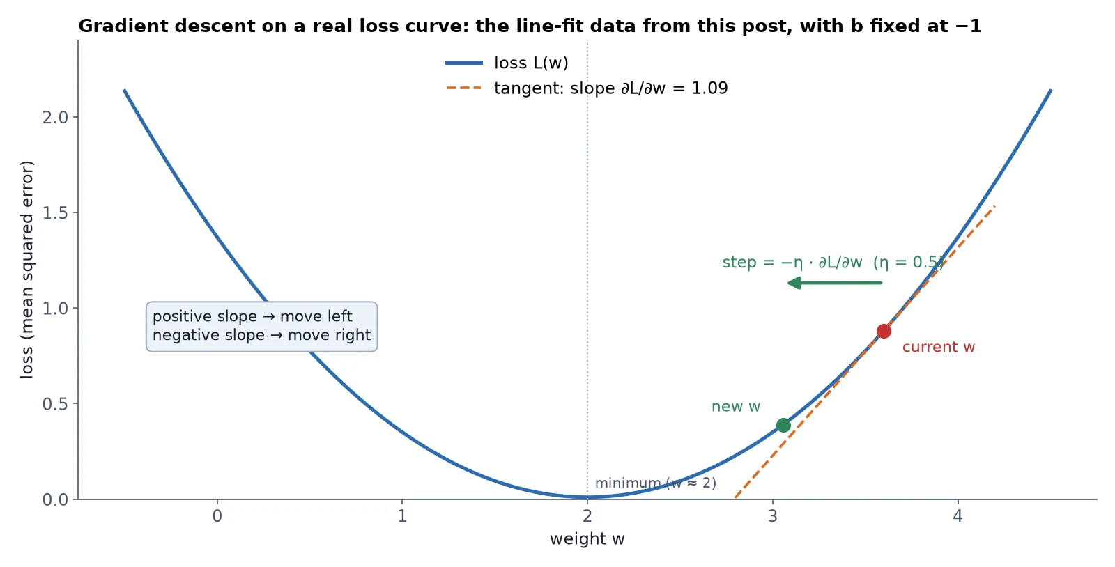
Computing \partial L / \partial w by hand for a transformer would take weeks and break every time you changed the model. Autograd computes it automatically, exactly, for any model you can write in PyTorch.
What you just built: The gradient descent update w \leftarrow w – \eta\,\partial L/\partial w, the rule every step of training follows.
Step 2/6: PyTorch Autograd in Five Lines
In this step: We ask PyTorch for our first gradient and meet requires_grad, grad_fn and leaf tensors.
import torch

x = torch.tensor(3.0, requires_grad=True)   # "track every op on x"
y = x ** 2 + 2 * x                            # y = x^2 + 2x
print(y)                                      # y remembers how it was made: grad_fn

y.backward()                                  # dy/dx, computed for us
print(x.grad)                                 # 2x + 2 at x=3 -> 8
print(x.is_leaf, y.is_leaf) # x was created by us; y by an optensor(15., grad_fn=<AddBackward0>)
tensor(8.)
True FalseThree new ideas are packed in here:
requires_grad=Truetells PyTorch to record every operation that usesx.ywas produced by an operation, so it carries agrad_fn(hereAddBackward0), a pointer to the node in the graph that created it.y.backward()computes \frac{dy}{dx} = 2x + 2 = 8 at x = 3 and stores it inx.grad.
x is a leaf tensor: we created it ourselves, so it sits at the edge of the graph. Gradients are stored on leaves. In a model, the leaves with requires_grad=True are the weights.
Note: In post 5, nn.Linear will create the weights for us as nn.Parameter objects, which are leaf tensors with requires_grad=True built in.
What you just built: Your first autograd gradient: dy/dx = 8 at x = 3, stored in x.grad.
Step 3/6: The Computational Graph and the Chain Rule
In this step: We watch PyTorch record a graph during the forward pass and replay it backwards, and check the result against the chain rule by hand.
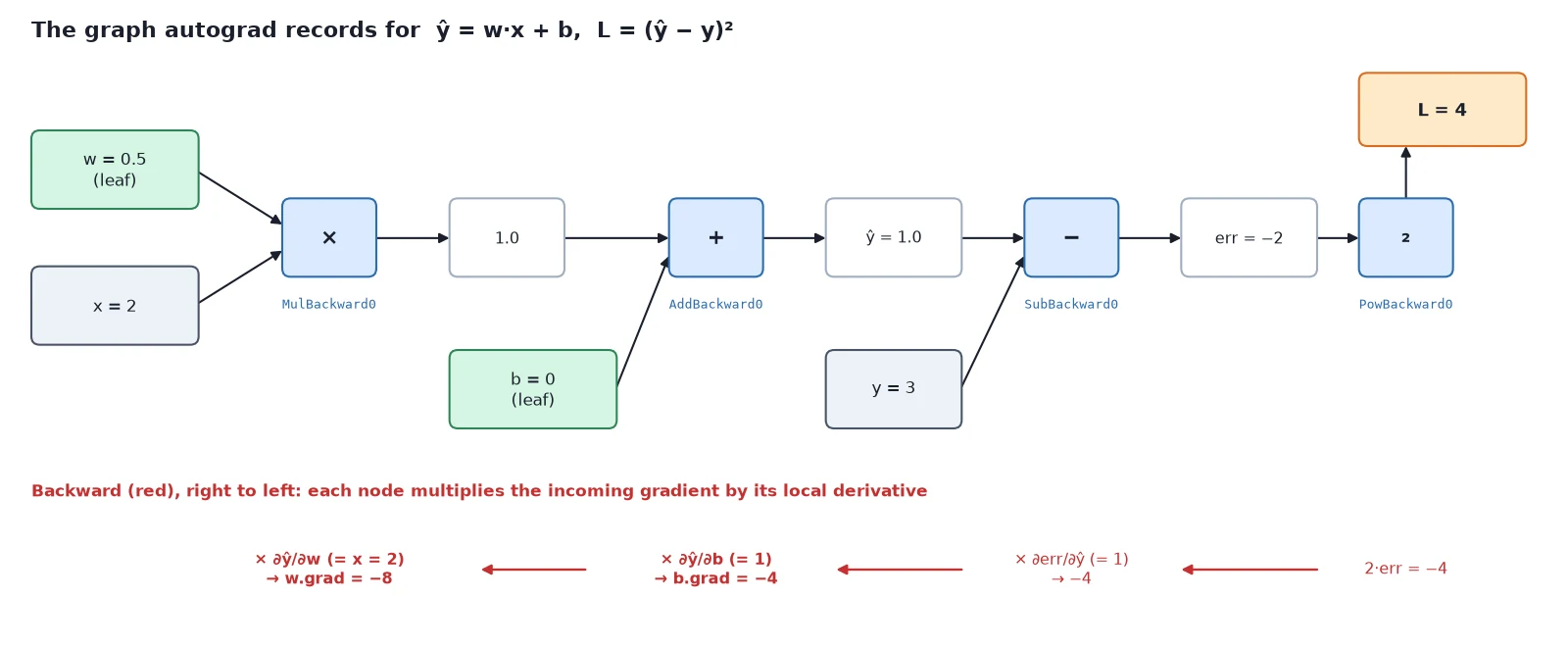
Here is a tiny version of what every training step does: one weight w, one bias b, one data point (x, y) = (2, 3), a prediction, and a squared-error loss.
import torch

w = torch.tensor(0.5, requires_grad=True)
b = torch.tensor(0.0, requires_grad=True)
x, y = torch.tensor(2.0), torch.tensor(3.0)   # one data point; no grad needed

y_hat = w * x + b            # prediction: 1.0
err = y_hat - y              # error: -2.0
loss = err ** 2              # squared error: 4.0

# Walk the recorded graph backwards from the loss, one node at a time.
node = loss.grad_fn
while node is not None:
    print(type(node).__name__)
    nxt = [n for n, _ in node.next_functions if n is not None and type(n).__name__ != "AccumulateGrad"]
    node = nxt[0] if nxt else None

loss.backward()
print("autograd:", w.grad.item(), b.grad.item())

# Chain rule by hand: dL/dw = 2*err*x, dL/db = 2*err*1
print("by hand: ", (2 * err * x).item(), (2 * err).item())PowBackward0
SubBackward0
AddBackward0
MulBackward0
autograd: -8.0 -4.0
by hand: -8.0 -4.0The forward pass built this chain: multiply, add, subtract, square. backward() walked it in reverse: PowBackward0 first, MulBackward0 last.
Why backward() works: the chain rule
Each operation in the graph only needs to know its own local derivative. The chain rule multiplies those local pieces along the path from the loss back to a weight:
\begin{gathered} \frac{\partial L}{\partial w} \;=\; \underbrace{\frac{\partial L}{\partial \text{err}}}_{2\,\text{err} \,=\, -4} \cdot \underbrace{\frac{\partial\, \text{err}}{\partial \hat y}}_{1} \cdot \underbrace{\frac{\partial \hat y}{\partial w}}_{x \,=\, 2} \;=\; -8 \\ \frac{\partial L}{\partial b} \;=\; -4 \cdot 1 \cdot \underbrace{1}_{\partial \hat y / \partial b} \;=\; -4 \end{gathered}That matches the autograd output exactly. Both gradients are negative, which means “increasing w or b would lower the loss”. That makes sense: the prediction (1.0) is below the target (3.0).
This is called reverse-mode automatic differentiation. Its big advantage: one backward pass gives the gradient for every weight at once, whether the model has 2 weights or 2 billion. The cost is roughly the same as one or two forward passes.
The computational graph and backward(): what, why, how
What it is: the machinery that gets the exact derivative of the loss with respect to every weight, without writing a single derivative by hand. Every layer we build later (attention, patch embeddings, the timestep embedding, RMSNorm…) gets its gradients this way for free.
Why it works: the chain rule. A huge model is just many small operations in a row, and each small operation knows its own local derivative (the derivative of x * w with respect to w is x; the derivative of u ** 2 is 2u). Multiplying local derivatives along the path from the loss back to a weight gives that weight’s gradient.
Going backwards means each intermediate result is reused for every weight that feeds into it, which is why one backward pass is enough for all of them.
How it works:
- Forward pass: for every operation on a tensor with
requires_grad=True, PyTorch creates a node (MulBackward0,AddBackward0, …), saves the inputs it will need, and links it to the nodes of its inputs. The result’sgrad_fnpoints at that node. loss.backward(): starting from \partial L / \partial L = 1, PyTorch visits the nodes in reverse order. Each node multiplies the incoming gradient by its local derivative and passes the result to its inputs.- Leaves: when the gradient reaches a leaf tensor (a weight), it is added to
.grad. - Cleanup: by default the graph is freed after
backward(). The next forward pass builds a fresh one. This “define-by-run” design is why you can use plain Pythonifandforinside a PyTorch model.
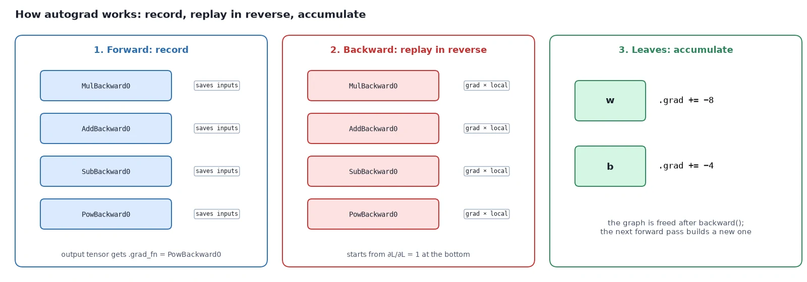
What you just built: A traced graph for \hat y = wx + b with gradients \partial L/\partial w = -8 and \partial L/\partial b = -4, confirmed by the chain rule.
Step 4/6: Gradients Accumulate: Why zero_grad() Exists
In this step: We see that backward() adds to .grad instead of overwriting it, and what goes wrong if you forget to reset it.
backward() does not overwrite .grad. It adds to it:
import torch

w = torch.tensor(1.0, requires_grad=True)

for i in range(3):
    loss = 3 * w          # d(loss)/dw = 3 every time
    loss.backward()
    print(f"after backward #{i + 1}: w.grad = {w.grad.item()}")

w.grad.zero_()            # what optimizer.zero_grad() does for every parameter
print("after zero_():", w.grad.item())after backward #1: w.grad = 3.0
after backward #2: w.grad = 6.0
after backward #3: w.grad = 9.0
after zero_(): 0.0This is a deliberate design choice. It lets you add up gradients from several small batches before taking one step (a trick called gradient accumulation, useful when a big batch does not fit in memory).
Watch out: In a normal training loop you must reset the gradients every step. Otherwise each update uses the sum of all past gradients, and the steps get bigger and bigger in stale directions.
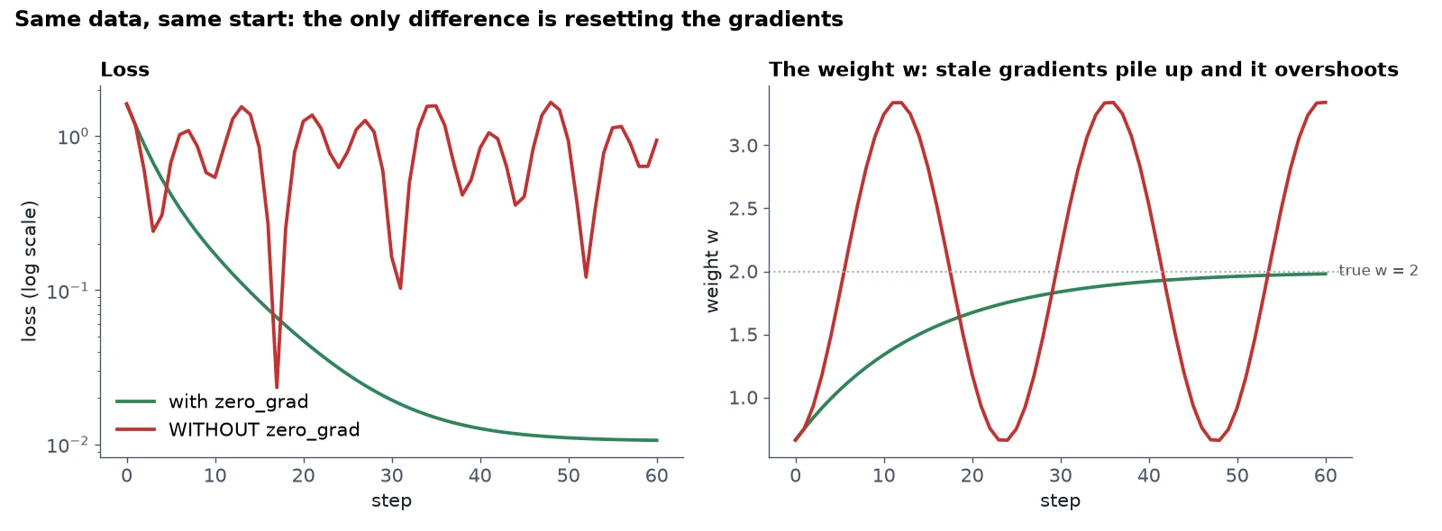
Here is the difference on a real fit (the full script is in step 6):
import torch

torch.manual_seed(0)
x = torch.linspace(-1, 1, 100)
y = 2 * x - 1 + 0.1 * torch.randn(100)

def train(zero_grad: bool, steps=60, lr=0.1):
    w = torch.randn(1, requires_grad=True)
    b = torch.zeros(1, requires_grad=True)
    for step in range(steps + 1):
        loss = ((w * x + b - y) ** 2).mean()
        loss.backward()
        with torch.no_grad():
            w -= lr * w.grad
            b -= lr * b.grad
        if zero_grad:
            w.grad.zero_(); b.grad.zero_()
        if step % 15 == 0:
            print(f"  step {step:2d} | loss {loss.item():9.4f}")

torch.manual_seed(1); print("with zero_grad:"); train(True)
torch.manual_seed(1); print("WITHOUT zero_grad:"); train(False)with zero_grad:
step 0 | loss 1.6124
step 15 | loss 0.0854
step 30 | loss 0.0194
step 45 | loss 0.0116
step 60 | loss 0.0106
WITHOUT zero_grad:
step 0 | loss 1.6124
step 15 | loss 0.8458
step 30 | loss 0.1642
step 45 | loss 0.4042
step 60 | loss 0.9394With zero_grad, the loss falls steadily. Without it, the loss drops at first, then bounces back up because each step is driven by a growing pile of old gradients.
That is why every training loop in this series, starting with the Trainer in post 5, opens each step with optimizer.zero_grad().
What you just built: Proof, on a real fit, that forgetting zero_grad() makes training unstable.
Step 5/6: torch.no_grad(): Turning Recording Off
In this step: We switch gradient recording off for evaluation, sampling and manual weight updates.
Recording the graph costs memory: PyTorch keeps intermediate values around so backward() can use them. When you don’t need gradients (evaluation, sampling images, or updating weights by hand), switch recording off:
import torch

w = torch.randn(256, 256, requires_grad=True)
x = torch.randn(64, 256)

y = x @ w
print("training mode:", y.requires_grad, y.grad_fn is not None)

with torch.no_grad():                 # inference / evaluation / sampling
    y = x @ w
print("inside no_grad:", y.requires_grad, y.grad_fn)

z = (x @ w).detach()                  # cut one tensor out of the graph
print("detached:", z.requires_grad)

@torch.no_grad()                      # same thing, as a decorator
def predict(inp):
    return inp @ w
print("decorated:", predict(x).requires_grad)training mode: True True
inside no_grad: False None
detached: False
decorated: Falsewith torch.no_grad():turns tracking off for a block of code. Results have nograd_fnand keep no intermediate values alive..detach()returns a tensor that shares the numbers but is cut out of the graph.@torch.no_grad()does the same as a decorator. TheTrainer.evaluatemethod in post 5 and TinyDiT’s sampler in post 9 both use it.
Why it works: In the weight update, no_grad is not just about memory: we don’t want “subtract the gradient” to become part of the graph we differentiate next time.
What you just built: Three ways to stop recording: with torch.no_grad(), .detach() and the @torch.no_grad() decorator.
Step 6/6: Fit a Line with Autograd and No Optimizer
In this step: We train our first model, a straight line, with autograd and a hand-written gradient descent loop.
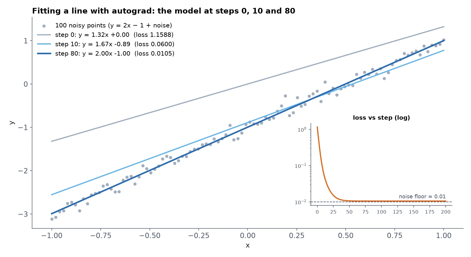
The data comes from the line y = 2x – 1 plus a little noise. The model is \hat y = wx + b, and we want autograd plus gradient descent to find w \approx 2 and b \approx -1. No nn.Module, no optimizer, just the raw loop.
This file goes in the repo as examples/fit_line.py. First, the noisy data and the two parameters autograd should track:
"""Fit y = w*x + b with nothing but tensors, autograd and a hand-written update (post 3).

No nn.Module, no optimizer yet. Run: python examples/fit_line.py
"""
import torch

torch.manual_seed(0)

# 1) Data: 100 points on the line y = 2x - 1, plus a little noise.
x = torch.linspace(-1, 1, 100)
y = 2 * x - 1 + 0.1 * torch.randn(100)

# 2) Parameters: leaf tensors that autograd should track.
w = torch.randn(1, requires_grad=True)
b = torch.zeros(1, requires_grad=True)Then the loop: forward, backward, update without recording, and reset the gradients:
lr = 0.1  # learning rate: how big each step is
for step in range(201):
    # Forward pass: PyTorch records every op into a graph.
    y_hat = w * x + b
    loss = ((y_hat - y) ** 2).mean()          # mean squared error

    # Backward pass: walk the graph, fill w.grad and b.grad.
    loss.backward()

    # Update: step against the gradient. no_grad() = "don't record this".
    with torch.no_grad():
        w -= lr * w.grad
        b -= lr * b.grad

    # Gradients ACCUMULATE (+=) on every backward(). Reset them, or the next
    # step adds this step's gradient on top. The Trainer in post 5 calls this
    # optimizer.zero_grad() at the start of every step for the same reason.
    w.grad.zero_()
    b.grad.zero_()

    if step % 40 == 0:
        print(f"step {step:3d} | loss {loss.item():.4f} | w {w.item():.3f} | b {b.item():.3f}")

print(f"learned: y = {w.item():.2f} x {b.item():+.2f} (true: y = 2.00 x -1.00)")step 0 | loss 1.1588 | w 1.369 | b -0.199
step 40 | loss 0.0111 | w 1.962 | b -0.996
step 80 | loss 0.0105 | w 1.998 | b -0.996
step 120 | loss 0.0105 | w 2.000 | b -0.996
step 160 | loss 0.0105 | w 2.000 | b -0.996
step 200 | loss 0.0105 | w 2.000 | b -0.996
learned: y = 2.00 x -1.00 (true: y = 2.00 x -1.00)It finds the line in about 80 steps. The loss settles at about 0.0105, not 0. That is the noise we added on purpose (0.1^2 = 0.01); no straight line can explain random noise.
The loss here is the mean squared error (MSE), which will come back as the flow-matching loss in post 8:
\begin{gathered} L(w, b) = \frac{1}{n}\sum_{i=1}^{n} \big(\underbrace{w x_i + b}_{\text{prediction } \hat y_i} - \underbrace{y_i}_{\text{target}}\big)^2 \\ \frac{\partial L}{\partial w} = \frac{2}{n}\sum_i (\hat y_i - y_i)\,x_i \qquad \frac{\partial L}{\partial b} = \frac{2}{n}\sum_i (\hat y_i - y_i) \end{gathered}You never wrote those two derivative formulas in code. Autograd derived them from the forward pass.
Every training loop in this series has exactly the same skeleton as this script:
- forward: compute the prediction and the loss;
- backward:
loss.backward()fills.gradfor every weight; - step: move each weight against its gradient;
- zero_grad: reset the gradients for the next step.
Note: In post 5 we swap step 3 for optimizer.step() (AdamW) and step 4 for optimizer.zero_grad(), and the two weights become a whole nn.Module. The skeleton stays the same.
What you just built: examples/fit_line.py, which recovers y = 2x – 1 from noisy data with the forward → backward → step → zero_grad loop.
Recap
requires_grad=Truemakes PyTorch record operations. Results carry agrad_fn. Leaves, like weights, receive.grad.backward()is the chain rule applied in reverse over the recorded graph. One pass gives every gradient.- Gradients accumulate. Reset them every step with
zero_grad(), or your steps grow and training goes unstable. - Use
torch.no_grad()(or.detach()) for evaluation, sampling and manual weight updates. - The training heartbeat is forward → loss → backward → step → zero_grad. We used it to fit y = 2x – 1 with plain tensors.
Next up: We need real data. In PyTorch DataLoader Explained: Datasets, Batches, and Image Folders we build the Dataset and DataLoader that feed CIFAR-10 images, or your own pictures, to TinyDiT in tidy (N, 3, 32, 32) batches.
Series: PyTorch Tutorial 2026 (14 posts)
- Post 1: PyTorch Tutorial 2026: From Tensors to Tiny Diffusion
- Post 2: PyTorch Tensors Explained: Shapes, Broadcasting, and Images as Arrays
- Post 3: PyTorch Autograd: How backward() Builds Gradients (you are here)
- Post 4: PyTorch DataLoader Explained: Datasets, Batches, and Image Folders
- Post 5: PyTorch nn.Module and the Training Loop: Layers, Loss, and Checkpoints
- Post 6: Attention and the Transformer Block in PyTorch
- Post 7: Patch Embeddings in PyTorch: How a Transformer Reads an Image
- Post 8: Flow Matching in PyTorch: Train a Model to Follow a Straight Line
- Post 9: Build a Tiny Diffusion Transformer in PyTorch (DiT from Scratch)
- Post 10: torch.compile, Mixed Precision, and SDPA: Speed Up TinyDiT
- Post 11: RMSNorm, QK-Norm, SwiGLU, and 2D RoPE in a Tiny DiT
- Post 12: adaLN-Zero and Classifier-Free Guidance in PyTorch
- Post 13: MMDiT Joint Attention in PyTorch: Two Streams, One Generator
- Post 14: Train and Sample Like 2026: Logit-Normal Steps, EMA, and Few-Step Flow
← Previous: Post 2: PyTorch Tensors Explained: Shapes, Broadcasting, and Images as Arrays
Next → Post 4: PyTorch DataLoader Explained: Datasets, Batches, and Image Folders