RMSNorm, QK-Norm, SwiGLU, and 2D RoPE in a Tiny DiT

In this post:

• Introduction
• Step 1/6: How We Measure "Better"
• Step 2/6: RMSNorm: Normalise Without Centring
• Step 3/6: QK-Norm: Keep Attention Scores in Check
• Step 4/6: SwiGLU: A Gated Feed-Forward Network
• Step 5/6: 2D RoPE: Positions as Rotations
• Step 6/6: The Before/After on TinyDiT
• Recap

Introduction

Welcome to the Expert half of the series. TinyDiT from Build a Tiny Diffusion Transformer in PyTorch (DiT from Scratch) is a 2023-style DiT: LayerNorm, a GELU feed-forward network, and learned position embeddings. The image models of 2024 to 2026 (Stable Diffusion 3, FLUX, and most open models since) keep the same skeleton but swap four small parts inside the block.

This post builds all four: RMSNorm, QK-norm, SwiGLU and 2D RoPE. In this PyTorch RMSNorm tutorial (and QK-norm, SwiGLU and RoPE tutorial), each part gets the same treatment: what it does, the code, a tiny test you can run, and then a measured before/after on TinyDiT.

No “trust me, it’s better”. We train every version with the same settings and report the real numbers, including the ones that don’t move.

Step 1/6: How We Measure “Better”

In this step: We fix the four numbers every run reports, and the seed gap that tells a real result from noise.

Every run below reports the same four numbers, computed the same way:

• Val MSE: the flow-matching loss on 2,000 CIFAR-10 test images, with fixed noise and fixed times, so every model gets exactly the same exam (the held-out loss from Build a Tiny Diffusion Transformer in PyTorch (DiT from Scratch)). Lower is better.
• Probe-FD: 1,000 samples (20 Euler steps) compared with real images using a small CIFAR-10 classifier’s features, the same idea as FID but with our own small network. It is not the FID you see in papers, so only compare it within this series. Lower is better.
• ms/step: training speed, measured while two runs share the CPU, so treat small differences as noise.
• Loss spikes: steps whose loss jumps above 1.5× the median of the previous 100 steps.

Step 2/6: RMSNorm: Normalise Without Centring

In this step: We replace LayerNorm with RMSNorm, check it against PyTorch’s own version, and time it.

LayerNorm (post 5) does two things to each token: it subtracts the mean, then divides by the standard deviation. RMSNorm (Zhang and Sennrich, Root Mean Square Layer Normalization, NeurIPS 2019) skips the first step and divides by the root mean square:

\begin{gathered} \operatorname{LN}(x) = \frac{x - \operatorname{mean}(x)}{\sqrt{\operatorname{var}(x) + \epsilon}} \\ \operatorname{RMSNorm}(x) = \frac{x}{\sqrt{\operatorname{mean}(x^2) + \epsilon}} \end{gathered}

The paper’s argument: the useful part of LayerNorm is the re-scaling, which keeps activations at a steady size. The re-centring adds work but little benefit.

Here’s ours, in tinydit/expert.py:

class RMSNorm(nn.Module):
    """y = x / sqrt(mean(x^2) + eps) * weight. No mean subtraction, no bias (Zhang & Sennrich, 2019)."""

    def __init__(self, dim: int, eps: float = 1e-6, elementwise_affine: bool = True):
        super().__init__()
        self.eps = eps
        self.weight = nn.Parameter(torch.ones(dim)) if elementwise_affine else None

    def forward(self, x: torch.Tensor) -> torch.Tensor:
        # Same maths as x * rsqrt(mean(x**2) + eps) * weight, but one fused PyTorch kernel.
        return F.rms_norm(x, (x.shape[-1],), self.weight, self.eps)

class RMSNorm(nn.Module):
    """y = x / sqrt(mean(x^2) + eps) * weight. No mean subtraction, no bias (Zhang & Sennrich, 2019)."""

    def __init__(self, dim: int, eps: float = 1e-6, elementwise_affine: bool = True):
        super().__init__()
        self.eps = eps
        self.weight = nn.Parameter(torch.ones(dim)) if elementwise_affine else None

    def forward(self, x: torch.Tensor) -> torch.Tensor:
        # Same maths as x * rsqrt(mean(x**2) + eps) * weight, but one fused PyTorch kernel.
        return F.rms_norm(x, (x.shape[-1],), self.weight, self.eps)

And a test next to nn.LayerNorm and PyTorch’s own nn.RMSNorm:

import time
import torch
from torch import nn
from tinydit.expert import RMSNorm

torch.manual_seed(0)
x = torch.randn(4, 64, 128) * 3 + 1                    # tokens with a non-zero mean
ln, rms = nn.LayerNorm(128, elementwise_affine=False), RMSNorm(128, elementwise_affine=False)
a, b = ln(x), rms(x)
print("LayerNorm output: mean %.3f, rms %.3f" % (a.mean(-1).abs().mean(), a.pow(2).mean(-1).sqrt().mean()))
print("RMSNorm   output: mean %.3f, rms %.3f" % (b.mean(-1).abs().mean(), b.pow(2).mean(-1).sqrt().mean()))
print("ours == torch.nn.RMSNorm:", torch.allclose(RMSNorm(128)(x), nn.RMSNorm(128, eps=1e-6)(x), atol=1e-6))

x = torch.randn(128, 64, 128)
for name, norm in [("LayerNorm", ln), ("RMSNorm", rms)]:
    for _ in range(10): norm(x)
    t0 = time.perf_counter()
    for _ in range(200): norm(x)
    print(f"{name:9s} {(time.perf_counter() - t0) / 200 * 1e3:.3f} ms per call (CPU, eager)")

import time
import torch
from torch import nn
from tinydit.expert import RMSNorm

torch.manual_seed(0)
x = torch.randn(4, 64, 128) * 3 + 1                    # tokens with a non-zero mean
ln, rms = nn.LayerNorm(128, elementwise_affine=False), RMSNorm(128, elementwise_affine=False)
a, b = ln(x), rms(x)
print("LayerNorm output: mean %.3f, rms %.3f" % (a.mean(-1).abs().mean(), a.pow(2).mean(-1).sqrt().mean()))
print("RMSNorm   output: mean %.3f, rms %.3f" % (b.mean(-1).abs().mean(), b.pow(2).mean(-1).sqrt().mean()))
print("ours == torch.nn.RMSNorm:", torch.allclose(RMSNorm(128)(x), nn.RMSNorm(128, eps=1e-6)(x), atol=1e-6))

x = torch.randn(128, 64, 128)
for name, norm in [("LayerNorm", ln), ("RMSNorm", rms)]:
    for _ in range(10): norm(x)
    t0 = time.perf_counter()
    for _ in range(200): norm(x)
    print(f"{name:9s} {(time.perf_counter() - t0) / 200 * 1e3:.3f} ms per call (CPU, eager)")

LayerNorm output: mean 0.000, rms 1.000
RMSNorm   output: mean 0.305, rms 1.000
ours == torch.nn.RMSNorm: True
LayerNorm 13.872 ms per call (CPU, eager)
RMSNorm   43.351 ms per call (CPU, eager)

LayerNorm’s outputs have mean 0 and size 1. RMSNorm’s outputs have size 1 but keep their mean. And our version matches torch.nn.RMSNorm exactly.

On a GPU, and with torch.compile, RMSNorm gets fused too, and that’s where its speed advantage shows up. Lesson: a “cheaper” formula is only cheaper if your library runs it as one operation. Always time it on your own hardware.

RMSNorm: what, why, how

What it is: a norm that keeps each token’s activations at a steady size, like LayerNorm.

Why it works: the re-scaling is what stabilises training; dropping the mean subtraction removes work and a bias parameter without losing that (Zhang and Sennrich, 2019).

How it works: x / sqrt(mean(x**2) + eps) * weight, one call: F.rms_norm(x, (D,), weight, eps). In TinyDiT: --set norm=rmsnorm.

Step 3/6: QK-Norm: Keep Attention Scores in Check

In this step: We normalise queries and keys before the dot product so attention scores can’t run away as weights grow.

Attention scores are dot products q \cdot k / \sqrt{d}. If the weights that produce q and k grow during training, the scores grow with the square of that growth, softmax saturates (one key gets almost all the weight), and its gradients nearly vanish. That’s a known cause of loss spikes in big transformers.

QK-norm applies an RMSNorm to q and to k (per head) just before the dot product, so their size can’t run away. ViT-22B (Dehghani et al., 2023) used it to train stably at scale, and SD3 (Esser et al., 2024) and FLUX use it in every attention layer.

import torch
from tinydit.expert import RMSNorm

torch.manual_seed(0)
q, k = torch.randn(64, 32), torch.randn(64, 32)       # 64 tokens, head_dim 32
qk_norm = RMSNorm(32)
for growth in [1, 4, 16]:                              # weights drifting bigger during training
    logits = (growth * q) @ (growth * k).T / 32 ** 0.5
    normed = qk_norm(growth * q) @ qk_norm(growth * k).T / 32 ** 0.5
    top = logits.softmax(-1).max(-1).values.mean()
    top_n = normed.softmax(-1).max(-1).values.mean()
    print(f"q,k x{growth:<2}: max |logit| {logits.abs().max():7.1f} -> top weight {top:.2f}"
          f"   | with QK-norm: max |logit| {normed.abs().max():5.1f} -> top weight {top_n:.2f}")

import torch
from tinydit.expert import RMSNorm

torch.manual_seed(0)
q, k = torch.randn(64, 32), torch.randn(64, 32)       # 64 tokens, head_dim 32
qk_norm = RMSNorm(32)
for growth in [1, 4, 16]:                              # weights drifting bigger during training
    logits = (growth * q) @ (growth * k).T / 32 ** 0.5
    normed = qk_norm(growth * q) @ qk_norm(growth * k).T / 32 ** 0.5
    top = logits.softmax(-1).max(-1).values.mean()
    top_n = normed.softmax(-1).max(-1).values.mean()
    print(f"q,k x{growth:<2}: max |logit| {logits.abs().max():7.1f} -> top weight {top:.2f}"
          f"   | with QK-norm: max |logit| {normed.abs().max():5.1f} -> top weight {top_n:.2f}")

q,k x1 : max |logit|     3.8 -> top weight 0.11   | with QK-norm: max |logit|   3.4 -> top weight 0.10
q,k x4 : max |logit|    60.5 -> top weight 0.90   | with QK-norm: max |logit|   3.4 -> top weight 0.10
q,k x16: max |logit|   968.8 -> top weight 1.00   | with QK-norm: max |logit|   3.4 -> top weight 0.10

Without QK-norm, making q and k 4× bigger makes the scores 16× bigger and attention becomes almost one-hot (top weight 0.90, then 1.00). With QK-norm the scores, and the attention pattern, don’t change.

In code it is two lines in our attention class:

class ModernAttention(MultiHeadAttention):
    """MultiHeadAttention + optional RMSNorm on q and k (per head) + optional 2D RoPE."""

    def __init__(self, dim: int, num_heads: int, use_sdpa: bool = True, qk_norm: bool = False):
        super().__init__(dim, num_heads, use_sdpa=use_sdpa)
        self.q_norm = RMSNorm(self.head_dim) if qk_norm else nn.Identity()
        self.k_norm = RMSNorm(self.head_dim) if qk_norm else nn.Identity()

    def qkv_heads(self, x: torch.Tensor, rope=None):
        q, k, v = self.split_heads(x)                       # (N, heads, L, head_dim)
        q, k = self.q_norm(q), self.k_norm(k)               # QK-norm (ViT-22B, FLUX)
        if rope is not None:
            q, k = apply_rope(q, *rope), apply_rope(k, *rope)
        return q, k, v

    def attend(self, q, k, v) -> torch.Tensor:
        n, _, l, _ = q.shape
        out = F.scaled_dot_product_attention(q, k, v) if self.use_sdpa else (
            torch.softmax(q @ k.transpose(-2, -1) * self.head_dim ** -0.5, -1) @ v)
        return out.transpose(1, 2).reshape(n, l, -1)

    def forward(self, x: torch.Tensor, rope=None) -> torch.Tensor:
        return self.proj(self.attend(*self.qkv_heads(x, rope)))

class ModernAttention(MultiHeadAttention):
    """MultiHeadAttention + optional RMSNorm on q and k (per head) + optional 2D RoPE."""

    def __init__(self, dim: int, num_heads: int, use_sdpa: bool = True, qk_norm: bool = False):
        super().__init__(dim, num_heads, use_sdpa=use_sdpa)
        self.q_norm = RMSNorm(self.head_dim) if qk_norm else nn.Identity()
        self.k_norm = RMSNorm(self.head_dim) if qk_norm else nn.Identity()

    def qkv_heads(self, x: torch.Tensor, rope=None):
        q, k, v = self.split_heads(x)                       # (N, heads, L, head_dim)
        q, k = self.q_norm(q), self.k_norm(k)               # QK-norm (ViT-22B, FLUX)
        if rope is not None:
            q, k = apply_rope(q, *rope), apply_rope(k, *rope)
        return q, k, v

    def attend(self, q, k, v) -> torch.Tensor:
        n, _, l, _ = q.shape
        out = F.scaled_dot_product_attention(q, k, v) if self.use_sdpa else (
            torch.softmax(q @ k.transpose(-2, -1) * self.head_dim ** -0.5, -1) @ v)
        return out.transpose(1, 2).reshape(n, l, -1)

    def forward(self, x: torch.Tensor, rope=None) -> torch.Tensor:
        return self.proj(self.attend(*self.qkv_heads(x, rope)))

QK-norm: what, why, how

What it is: two small norms that prevent attention scores from growing out of control.

Why it works: normalised q and k have a fixed size, so q \cdot k is bounded and softmax can’t saturate just because weights grew (Dehghani et al., 2023; used in SD3 and FLUX).

How it works: two per-head RMSNorms, applied to q and k after the QKV split and before RoPE and attention. In TinyDiT: --set qk_norm=true.

Step 4/6: SwiGLU: A Gated Feed-Forward Network

In this step: We swap the GELU feed-forward network for a gated SwiGLU with the same parameter count.

Our FFN was Linear → GELU → Linear. SwiGLU (Shazeer, GLU Variants Improve Transformer, 2020) uses two parallel projections, a “gate” and a “value”, and multiplies them:

\begin{gathered} \operatorname{FFN}_{\text{GELU}}(x) = W_2\,\operatorname{GELU}(W_1 x) \\ \operatorname{SwiGLU}(x) = W_3\big(\operatorname{SiLU}(W_1 x) \odot W_2 x\big) \end{gathered}

The gate decides, feature by feature, how much of the value to let through. Three matrices instead of two would mean more parameters, so the standard trick (used by LLaMA too) is to shrink the hidden size to \tfrac{2}{3} of 4D.

Then the parameter count is the same, and any difference we measure comes from the design, not from size:

class SwiGLU(nn.Module):
    """Gated FFN: w3( SiLU(w1 x) * (w2 x) ) (Shazeer, 2020).

    hidden = 2/3 * mlp_ratio * dim, so the parameter count matches the GELU FeedForward
    (3 matrices of dim x hidden instead of 2 of dim x 4*dim).
    """

    def __init__(self, dim: int, mlp_ratio: float = 4.0):
        super().__init__()
        hidden = int(2 * mlp_ratio * dim / 3)
        self.w1 = nn.Linear(dim, hidden)     # gate
        self.w2 = nn.Linear(dim, hidden)     # value
        self.w3 = nn.Linear(hidden, dim)     # back to dim

    def forward(self, x: torch.Tensor) -> torch.Tensor:
        return self.w3(F.silu(self.w1(x)) * self.w2(x))

class SwiGLU(nn.Module):
    """Gated FFN: w3( SiLU(w1 x) * (w2 x) ) (Shazeer, 2020).

    hidden = 2/3 * mlp_ratio * dim, so the parameter count matches the GELU FeedForward
    (3 matrices of dim x hidden instead of 2 of dim x 4*dim).
    """

    def __init__(self, dim: int, mlp_ratio: float = 4.0):
        super().__init__()
        hidden = int(2 * mlp_ratio * dim / 3)
        self.w1 = nn.Linear(dim, hidden)     # gate
        self.w2 = nn.Linear(dim, hidden)     # value
        self.w3 = nn.Linear(hidden, dim)     # back to dim

    def forward(self, x: torch.Tensor) -> torch.Tensor:
        return self.w3(F.silu(self.w1(x)) * self.w2(x))

Check the parameter count against the GELU FFN:

import torch
from tinydit.layers import FeedForward
from tinydit.expert import SwiGLU

gelu, swiglu = FeedForward(128, mlp_ratio=4.0), SwiGLU(128, mlp_ratio=4.0)
count = lambda m: sum(p.numel() for p in m.parameters())
print(f"GELU FFN : 128 -> {gelu.fc1.out_features} -> 128   | {count(gelu):,} parameters")
print(f"SwiGLU   : 128 -> 2 x {swiglu.w1.out_features} -> 128 | {count(swiglu):,} parameters")
x = torch.randn(2, 64, 128)
print("same input/output shape:", gelu(x).shape == swiglu(x).shape == x.shape)

import torch
from tinydit.layers import FeedForward
from tinydit.expert import SwiGLU

gelu, swiglu = FeedForward(128, mlp_ratio=4.0), SwiGLU(128, mlp_ratio=4.0)
count = lambda m: sum(p.numel() for p in m.parameters())
print(f"GELU FFN : 128 -> {gelu.fc1.out_features} -> 128   | {count(gelu):,} parameters")
print(f"SwiGLU   : 128 -> 2 x {swiglu.w1.out_features} -> 128 | {count(swiglu):,} parameters")
x = torch.randn(2, 64, 128)
print("same input/output shape:", gelu(x).shape == swiglu(x).shape == x.shape)

GELU FFN : 128 -> 512 -> 128   | 131,712 parameters
SwiGLU   : 128 -> 2 x 341 -> 128 | 131,754 parameters
same input/output shape: True

SwiGLU: what, why, how

What it is: the feed-forward half of every block, with a learned gate.

Why it works: multiplying a gate by a value lets each feature be switched on or off by the input, which proved more expressive per parameter in Shazeer’s language-model tests.

How it works: w3(silu(w1(x)) * w2(x)) with hidden size \tfrac{2}{3} \cdot 4D, so it has the same parameters as the GELU FFN. In TinyDiT: --set mlp=swiglu.

Step 5/6: 2D RoPE: Positions as Rotations

In this step: We replace the learned position table with 2D rotary embeddings and check the relative-position property in code.

In post 7 we added a learned row vector and column vector to every patch token. Rotary position embeddings (RoPE; Su et al., RoFormer, 2021) work differently: they leave the tokens alone and instead rotate each query and key by an angle that depends on its position.

Rotate q by position m and k by position n, and their dot product only depends on the difference m – n:

\langle R_m q,\; R_n k \rangle = \langle q,\; R_{n-m}\, k \rangle

So attention sees relative positions (“2 patches to the right”) for free. For images we use 2D RoPE (as in FLUX and Heo et al., Rotary Position Embedding for Vision Transformer, ECCV 2024): half of each head’s features rotate with the patch’s row, the other half with its column.

Each pair of features turns at its own speed, from fast to slow, like the timestep waves in post 9:

def rope_2d(grid_size: int, head_dim: int, base: float = 100.0, n_prefix: int = 0):
    """cos, sin tables (L, head_dim) for 2D rotary embeddings on a row-major grid.

    The first half of each head's features rotates with the patch ROW, the second half with the
    COLUMN. Each feature pair (2i, 2i+1) turns by angle pos * base^(-i / (head_dim/4)).
    n_prefix extra tokens (condition tokens, post 13) get angle 0, i.e. no rotation.
    """
    quarter = head_dim // 4                                       # pairs per axis
    inv_freq = base ** (-torch.arange(quarter, dtype=torch.float32) / quarter)
    idx = torch.arange(grid_size * grid_size)
    rows, cols = (idx // grid_size).float(), (idx % grid_size).float()
    angles = torch.cat([rows[:, None] * inv_freq, cols[:, None] * inv_freq], dim=-1)   # (L, head_dim/2)
    if n_prefix:
        angles = torch.cat([torch.zeros(n_prefix, angles.shape[1]), angles])
    angles = angles.repeat_interleave(2, dim=-1)                  # one angle per pair -> (L, head_dim)
    return angles.cos(), angles.sin()


def apply_rope(x: torch.Tensor, cos: torch.Tensor, sin: torch.Tensor) -> torch.Tensor:
    """Rotate each pair (x_2i, x_2i+1) by its angle. x (N, heads, L, head_dim)."""
    x_pairs = x.reshape(*x.shape[:-1], -1, 2)
    rotated = torch.stack([-x_pairs[..., 1], x_pairs[..., 0]], dim=-1).reshape(x.shape)   # (-x2, x1)
    return x * cos + rotated * sin

def rope_2d(grid_size: int, head_dim: int, base: float = 100.0, n_prefix: int = 0):
    """cos, sin tables (L, head_dim) for 2D rotary embeddings on a row-major grid.

    The first half of each head's features rotates with the patch ROW, the second half with the
    COLUMN. Each feature pair (2i, 2i+1) turns by angle pos * base^(-i / (head_dim/4)).
    n_prefix extra tokens (condition tokens, post 13) get angle 0, i.e. no rotation.
    """
    quarter = head_dim // 4                                       # pairs per axis
    inv_freq = base ** (-torch.arange(quarter, dtype=torch.float32) / quarter)
    idx = torch.arange(grid_size * grid_size)
    rows, cols = (idx // grid_size).float(), (idx % grid_size).float()
    angles = torch.cat([rows[:, None] * inv_freq, cols[:, None] * inv_freq], dim=-1)   # (L, head_dim/2)
    if n_prefix:
        angles = torch.cat([torch.zeros(n_prefix, angles.shape[1]), angles])
    angles = angles.repeat_interleave(2, dim=-1)                  # one angle per pair -> (L, head_dim)
    return angles.cos(), angles.sin()


def apply_rope(x: torch.Tensor, cos: torch.Tensor, sin: torch.Tensor) -> torch.Tensor:
    """Rotate each pair (x_2i, x_2i+1) by its angle. x (N, heads, L, head_dim)."""
    x_pairs = x.reshape(*x.shape[:-1], -1, 2)
    rotated = torch.stack([-x_pairs[..., 1], x_pairs[..., 0]], dim=-1).reshape(x.shape)   # (-x2, x1)
    return x * cos + rotated * sin

Now check that the score depends only on the relative offset:

import torch
from tinydit.expert import rope_2d, apply_rope

cos, sin = rope_2d(grid_size=8, head_dim=32)         # one angle per (token, feature pair)
print("tables:", tuple(cos.shape), "(64 tokens x 32 features)")

torch.manual_seed(0)
q, k = torch.randn(32), torch.randn(32)
def score(row_q, col_q, row_k, col_k):
    """q.k after rotating q to grid slot (row_q, col_q) and k to slot (row_k, col_k)."""
    iq, ik = row_q * 8 + col_q, row_k * 8 + col_k
    qr = apply_rope(q.expand(1, 1, 64, 32), cos, sin)[0, 0, iq]
    kr = apply_rope(k.expand(1, 1, 64, 32), cos, sin)[0, 0, ik]
    return (qr @ kr).item()

print("same offset (1 down, 2 right), different places:")
for (r, c) in [(0, 0), (3, 4), (6, 5)]:
    print(f"  q at ({r},{c}), k at ({r + 1},{c + 2}): score {score(r, c, r + 1, c + 2):+.4f}")
print("different offset (3 down, 0 right):  score", f"{score(0, 0, 3, 0):+.4f}")
print("rotation keeps lengths:", torch.allclose(apply_rope(q.expand(1, 1, 64, 32), cos, sin).norm(dim=-1), q.norm().expand(1, 1, 64)))

import torch
from tinydit.expert import rope_2d, apply_rope

cos, sin = rope_2d(grid_size=8, head_dim=32)         # one angle per (token, feature pair)
print("tables:", tuple(cos.shape), "(64 tokens x 32 features)")

torch.manual_seed(0)
q, k = torch.randn(32), torch.randn(32)
def score(row_q, col_q, row_k, col_k):
    """q.k after rotating q to grid slot (row_q, col_q) and k to slot (row_k, col_k)."""
    iq, ik = row_q * 8 + col_q, row_k * 8 + col_k
    qr = apply_rope(q.expand(1, 1, 64, 32), cos, sin)[0, 0, iq]
    kr = apply_rope(k.expand(1, 1, 64, 32), cos, sin)[0, 0, ik]
    return (qr @ kr).item()

print("same offset (1 down, 2 right), different places:")
for (r, c) in [(0, 0), (3, 4), (6, 5)]:
    print(f"  q at ({r},{c}), k at ({r + 1},{c + 2}): score {score(r, c, r + 1, c + 2):+.4f}")
print("different offset (3 down, 0 right):  score", f"{score(0, 0, 3, 0):+.4f}")
print("rotation keeps lengths:", torch.allclose(apply_rope(q.expand(1, 1, 64, 32), cos, sin).norm(dim=-1), q.norm().expand(1, 1, 64)))

tables: (64, 32) (64 tokens x 32 features)
same offset (1 down, 2 right), different places:
  q at (0,0), k at (1,2): score +2.0566
  q at (3,4), k at (4,6): score +2.0566
  q at (6,5), k at (7,7): score +2.0566
different offset (3 down, 0 right):  score -3.3432
rotation keeps lengths: True

Three different query/key pairs, all “1 down, 2 right” of each other, get exactly the same score (+2.0566). Change the offset and the score changes. That’s the relative-position property, checked in code.

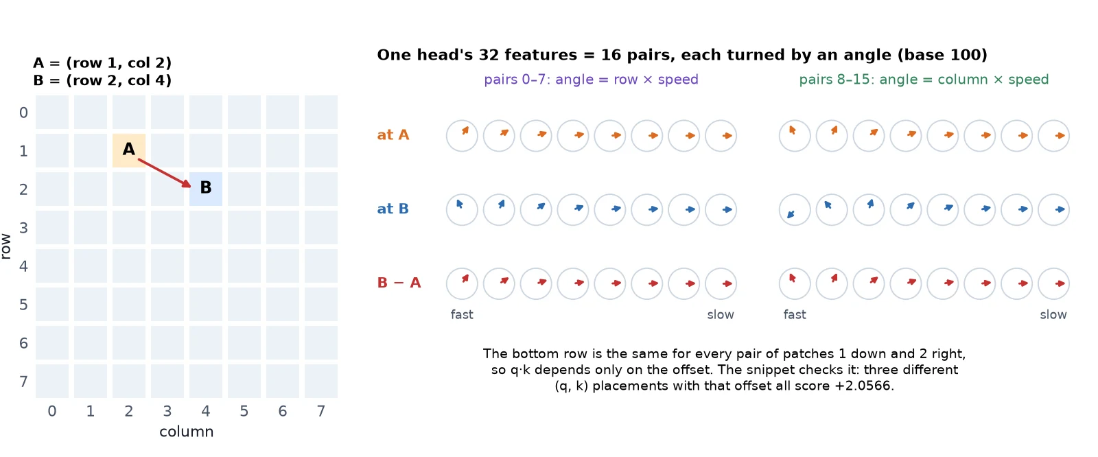
2D RoPE: what, why, how

What it is: a way of telling attention where each patch is.

Why it works: rotating q and k by position-dependent angles makes their dot product depend only on the relative position, and it adds no parameters (Su et al., 2021; 2D version as in FLUX).

How it works: precompute cos/sin tables for the 8×8 grid (row angles for half the features, column angles for the other half), then q*cos + rotate_half(q)*sin, same for k. The learned position table is removed. In TinyDiT: --set pos=rope2d.

Step 6/6: The Before/After on TinyDiT

In this step: We train seven runs that differ by one switch each, stress-test QK-norm at a high learning rate, and time every variant fairly.

Now the real test. Seven training runs, identical except for one switch each (the baseline twice, with two seeds). Every number below is read from the runs’ metrics.json files by this script:

import json
from pathlib import Path

runs = {"baseline (seed 0)": "p11_base_s0", "baseline (seed 1)": "p11_base_s1", "+ RMSNorm": "p11_rmsnorm",
        "+ QK-norm": "p11_qknorm", "+ SwiGLU": "p11_swiglu", "+ 2D RoPE": "p11_rope", "all four": "p11_all"}
m = {k: json.loads(Path(f"../runs/{v}/metrics.json").read_text()) for k, v in runs.items()}
print(f"{'run':18s} {'params':>9s} {'val MSE':>8s} {'probe-FD':>9s} {'ms/step':>8s} {'spikes':>6s}")
for k, r in m.items():
    print(f"{k:18s} {r['params']:9,d} {r['raw']['val_mse']:8.4f} {r['raw']['uncond']['probe_fd']:9.1f} "
          f"{1000 / r['it_per_s']:8.1f} {r['loss_spikes']:6d}")
base = [m["baseline (seed 0)"]["raw"]["val_mse"], m["baseline (seed 1)"]["raw"]["val_mse"]]
print(f"\nseed-to-seed difference of the baseline: {abs(base[0] - base[1]):.4f} (val MSE)")

print("\nhigh learning rate (2e-3, about 7x the default):")
for k, v in [("baseline", "p11_base_lr2e3"), ("+ QK-norm", "p11_qknorm_lr2e3")]:
    r = json.loads(Path(f"../runs/{v}/metrics.json").read_text())
    print(f"  {k:10s} val MSE {r['raw']['val_mse']:.4f} | probe-FD {r['raw']['uncond']['probe_fd']:.1f} | "
          f"loss spikes {r['loss_spikes']} | loss curve {[c[1] for c in r['curve'][::4]]}")

import json
from pathlib import Path

runs = {"baseline (seed 0)": "p11_base_s0", "baseline (seed 1)": "p11_base_s1", "+ RMSNorm": "p11_rmsnorm",
        "+ QK-norm": "p11_qknorm", "+ SwiGLU": "p11_swiglu", "+ 2D RoPE": "p11_rope", "all four": "p11_all"}
m = {k: json.loads(Path(f"../runs/{v}/metrics.json").read_text()) for k, v in runs.items()}
print(f"{'run':18s} {'params':>9s} {'val MSE':>8s} {'probe-FD':>9s} {'ms/step':>8s} {'spikes':>6s}")
for k, r in m.items():
    print(f"{k:18s} {r['params']:9,d} {r['raw']['val_mse']:8.4f} {r['raw']['uncond']['probe_fd']:9.1f} "
          f"{1000 / r['it_per_s']:8.1f} {r['loss_spikes']:6d}")
base = [m["baseline (seed 0)"]["raw"]["val_mse"], m["baseline (seed 1)"]["raw"]["val_mse"]]
print(f"\nseed-to-seed difference of the baseline: {abs(base[0] - base[1]):.4f} (val MSE)")

print("\nhigh learning rate (2e-3, about 7x the default):")
for k, v in [("baseline", "p11_base_lr2e3"), ("+ QK-norm", "p11_qknorm_lr2e3")]:
    r = json.loads(Path(f"../runs/{v}/metrics.json").read_text())
    print(f"  {k:10s} val MSE {r['raw']['val_mse']:.4f} | probe-FD {r['raw']['uncond']['probe_fd']:.1f} | "
          f"loss spikes {r['loss_spikes']} | loss curve {[c[1] for c in r['curve'][::4]]}")

run                   params  val MSE  probe-FD  ms/step spikes
baseline (seed 0)  1,152,176   0.2562      72.2    149.5      0
baseline (seed 1)  1,152,176   0.2527      70.5    148.6      0
+ RMSNorm          1,152,176   0.2559      71.7    177.6      0
+ QK-norm          1,152,432   0.2499      75.0    192.7      0
+ SwiGLU           1,152,344   0.2564      77.7    231.5      0
+ 2D RoPE          1,150,128   0.2289      63.9    246.9      0
all four           1,150,552   0.2266      62.3    357.1      0

seed-to-seed difference of the baseline: 0.0035 (val MSE)

high learning rate (2e-3, about 7x the default):
  baseline   val MSE 0.2085 | probe-FD 46.4 | loss spikes 0 | loss curve [0.39736, 0.24498, 0.21672, 0.20865]
  + QK-norm  val MSE 0.2069 | probe-FD 42.1 | loss spikes 0 | loss curve [0.39411, 0.24116, 0.21273, 0.20661]

What the numbers say, honestly:

• 2D RoPE is the one clear winner on TinyDiT. Its loss pulled ahead from step 750 and stayed ahead, and its samples score better too. Relative positions seem to matter a lot when a small model has to learn image structure from scratch in a few thousand steps.
• RMSNorm and SwiGLU made no measurable difference in quality at this size. That’s not a contradiction of the papers: RMSNorm’s main selling point is speed and simplicity, and SwiGLU’s gains were measured on much larger language models trained far longer. A 1.15M-parameter model trained for 4,000 steps can’t show a 1 to 2% effect through a seed gap of about 1.4%.
• QK-norm gave a gain barely above the seed noise, and a slightly worse probe-FD. Its real job is stability at scale, which we test next.
• All four together were about as good as RoPE alone. The other three didn’t hurt, so a modern block costs us nothing, but on this budget RoPE does the work.
• No run had a single loss spike (0 for all), so at this learning rate, stability was never a problem for the baseline.

A stress test for QK-norm: turn up the learning rate

QK-norm is meant to stop training from blowing up, and our baseline never blew up. So we made it harder: the same baseline and QK-norm runs again, but with a learning rate of 2e-3, about 7× the default.

A big learning rate makes weights grow faster, which is exactly what QK-norm protects against. The last two lines of the script output above are these runs:

Two honest findings:

• Neither run spiked. At 1.15M parameters and 4,000 steps, even a 7× learning rate doesn’t make attention scores run away, so QK-norm had nothing to rescue. Its val MSE gain (0.0016) is smaller than our seed gap (0.0035). Its probe-FD is better by 4.3, which is promising, but we only have one seed for it, so we call it “no harm, maybe a small help”. The stability benefit that ViT-22B and SD3 report shows up in models thousands of times bigger, trained much longer.
• The learning rate itself mattered more than any layer in this post. Both runs at 2e-3 beat every run at 3e-4 by a wide margin (val MSE 0.21 vs 0.23 to 0.26). Our default 3e-4 is a safe choice for big models, but too cautious for a tiny one.

A fair speed comparison

The ms/step column above was measured while other runs shared the CPU, and the load changed during the session, so it is not a fair speed comparison. Here’s a fair one: every variant timed in the same process, taking turns step by step, so any background load slows them all equally:

import time
import torch
from tinydit.expert import ExpertConfig, ExpertTinyDiT
from tinydit.flow import flow_matching_loss

torch.manual_seed(0)
torch.set_num_threads(2)
x = torch.randn(64, 3, 32, 32)
variants = {"baseline": {}, "+ RMSNorm": dict(norm="rmsnorm"), "+ QK-norm": dict(qk_norm=True),
            "+ SwiGLU": dict(mlp="swiglu"), "+ 2D RoPE": dict(pos="rope2d"),
            "all four": dict(norm="rmsnorm", qk_norm=True, mlp="swiglu", pos="rope2d")}
models = {k: ExpertTinyDiT(ExpertConfig(dim=128, depth=4, num_heads=4, **v)) for k, v in variants.items()}
opts = {k: torch.optim.AdamW(m.parameters(), lr=3e-4) for k, m in models.items()}
times = {k: [] for k in models}
for rnd in range(12):                  # take turns, so a busy CPU slows every variant equally
    for name, model in models.items():
        t0 = time.perf_counter()
        opts[name].zero_grad()
        flow_matching_loss(model, (x, None)).backward()
        opts[name].step()
        if rnd >= 2:                   # first 2 rounds are warm-up
            times[name].append(time.perf_counter() - t0)
base = sorted(times["baseline"])[5]
for name, ts in times.items():
    med = sorted(ts)[5]
    print(f"{name:10s} {med * 1000:6.1f} ms per training step | {med / base:.2f}x baseline")

import time
import torch
from tinydit.expert import ExpertConfig, ExpertTinyDiT
from tinydit.flow import flow_matching_loss

torch.manual_seed(0)
torch.set_num_threads(2)
x = torch.randn(64, 3, 32, 32)
variants = {"baseline": {}, "+ RMSNorm": dict(norm="rmsnorm"), "+ QK-norm": dict(qk_norm=True),
            "+ SwiGLU": dict(mlp="swiglu"), "+ 2D RoPE": dict(pos="rope2d"),
            "all four": dict(norm="rmsnorm", qk_norm=True, mlp="swiglu", pos="rope2d")}
models = {k: ExpertTinyDiT(ExpertConfig(dim=128, depth=4, num_heads=4, **v)) for k, v in variants.items()}
opts = {k: torch.optim.AdamW(m.parameters(), lr=3e-4) for k, m in models.items()}
times = {k: [] for k in models}
for rnd in range(12):                  # take turns, so a busy CPU slows every variant equally
    for name, model in models.items():
        t0 = time.perf_counter()
        opts[name].zero_grad()
        flow_matching_loss(model, (x, None)).backward()
        opts[name].step()
        if rnd >= 2:                   # first 2 rounds are warm-up
            times[name].append(time.perf_counter() - t0)
base = sorted(times["baseline"])[5]
for name, ts in times.items():
    med = sorted(ts)[5]
    print(f"{name:10s} {med * 1000:6.1f} ms per training step | {med / base:.2f}x baseline")

baseline    119.2 ms per training step | 1.00x baseline
+ RMSNorm   122.5 ms per training step | 1.03x baseline
+ QK-norm   151.3 ms per training step | 1.27x baseline
+ SwiGLU    118.4 ms per training step | 0.99x baseline
+ 2D RoPE   134.8 ms per training step | 1.13x baseline
all four    175.0 ms per training step | 1.47x baseline

On this CPU, SwiGLU costs nothing (same parameters, same speed) and RMSNorm costs about 3% (for the kernel reason we saw in step 2). The two components that do extra work per attention call are slower: QK-norm adds two normalisations per layer (+27 to 29%), and RoPE adds the rotations (+13 to 17%).

All four together cost about 1.5× per step. Those small elementwise operations are exactly what torch.compile fuses on a GPU, so the overhead there is much smaller, but we haven’t measured it, so we won’t quote a number. For TinyDiT, RoPE’s quality gain is well worth its cost.

Recap

• The four parts of a 2024 to 2026 transformer block are each a few lines of PyTorch: RMSNorm (F.rms_norm), QK-norm (two RMSNorms on q and k), SwiGLU (a gated FFN with the same parameter count) and 2D RoPE (rotate q and k by row and column angles).
• Each one passed a small test you can run: RMSNorm matches torch.nn.RMSNorm, QK-norm keeps attention scores fixed when q and k grow 16×, SwiGLU matches the GELU FFN’s size, and RoPE gives the same score for the same relative offset.
• Measured on TinyDiT (val MSE, lower is better; seed gap 0.0035): 2D RoPE 0.2289 vs 0.2562 baseline, a clear win; QK-norm 0.2499, a small gain at most; RMSNorm 0.2559 and SwiGLU 0.2564, no change at this scale.
• Even at a 7× learning rate no run had a loss spike, so QK-norm’s stability benefit doesn’t show up in a 1.15M-parameter model. The bigger learning rate itself improved val MSE to about 0.21.
• On this CPU, RMSNorm was slower than LayerNorm, not faster. Speed claims depend on your hardware and kernels, so time them yourself.
• From here on, TinyDiT uses 2D RoPE + QK-norm.

Next up: In adaLN-Zero and Classifier-Free Guidance in PyTorch, TinyDiT learns to follow instructions: class labels, classifier-free guidance, and the adaLN-Zero initialisation that DiT found works best.

← Previous: Post 10: torch.compile, Mixed Precision, and SDPA: Speed Up TinyDiT
Next → Post 12: adaLN-Zero and Classifier-Free Guidance in PyTorch