Build a Tiny Diffusion Transformer in PyTorch (DiT from Scratch)
Where you are: Post 9 of 14 in PyTorch Tutorial 2026 · about 12 min read
What you’ll build: tinydit/model.py: a timestep embedding, adaptive LayerNorm, DiTBlock, FinalLayer and the full TinyDiT, trained on CIFAR-10 to generate its first images, plus two honest scores for every later comparison.
You’ll need: Post 4 (loaders), Post 5 (Trainer), Post 6 (attention), Post 7 (patches) and Post 8 (flow-matching loss and sampler).
In this post:
- Introduction
- Step 1/5: The Timestep Embedding
- Step 2/5: Adaptive Layer Norm (adaLN)
- Step 3/5: PyTorch DiT: Putting TinyDiT Together
- Step 4/5: Train TinyDiT on CIFAR-10
- Step 5/5: How Good Are These Samples, Honestly?
- Recap
Series: PyTorch Tutorial 2026 (14 posts)
- Post 1: PyTorch Tutorial 2026: From Tensors to Tiny Diffusion
- Post 2: PyTorch Tensors Explained: Shapes, Broadcasting, and Images as Arrays
- Post 3: PyTorch Autograd: How backward() Builds Gradients
- Post 4: PyTorch DataLoader Explained: Datasets, Batches, and Image Folders
- Post 5: PyTorch nn.Module and the Training Loop: Layers, Loss, and Checkpoints
- Post 6: Attention and the Transformer Block in PyTorch
- Post 7: Patch Embeddings in PyTorch: How a Transformer Reads an Image
- Post 8: Flow Matching in PyTorch: Train a Model to Follow a Straight Line
- Post 9: Build a Tiny Diffusion Transformer in PyTorch (DiT from Scratch) (you are here)
- Post 10: torch.compile, Mixed Precision, and SDPA: Speed Up TinyDiT
- Post 11: RMSNorm, QK-Norm, SwiGLU, and 2D RoPE in a Tiny DiT
- Post 12: adaLN-Zero and Classifier-Free Guidance in PyTorch
- Post 13: MMDiT Joint Attention in PyTorch: Two Streams, One Generator
- Post 14: Train and Sample Like 2026: Logit-Normal Steps, EMA, and Few-Step Flow
Introduction
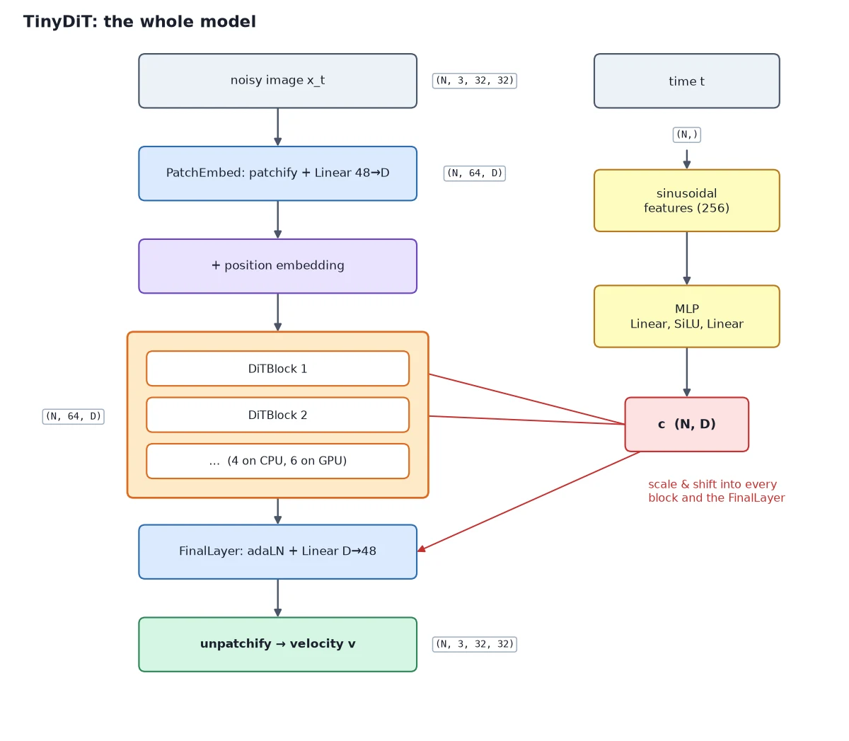
This is the post where our code finally makes pictures. We take the pieces from the last five posts (patch embeddings, transformer blocks, the flow-matching loss and the Euler sampler), add the one thing that’s missing, a way for the model to know the time t, and assemble a small Diffusion Transformer (DiT).
In this PyTorch DiT tutorial we build TinyDiT from scratch, train it on CIFAR-10, and generate our first images from pure noise. The images will be rough. We’ll look at them honestly and measure exactly how rough, because this model is the “before” that every Expert post improves on.
In Flow Matching in PyTorch: Train a Model to Follow a Straight Line we trained a tiny MLP to turn noise into two moons, and it read the time as a raw extra number. That’s fine for 2D points, but a transformer needs a richer signal. Today’s two new layers, a timestep embedding and adaptive layer norm (adaLN), solve that, and they are exactly what DiT (Peebles and Xie, Scalable Diffusion Models with Transformers, ICCV 2023) uses.
Note: CPU settings used in this post: dim 128, depth 4, 4 heads (1.15M parameters), batch 128, 6,000 steps, about 11 minutes on an 8-core CPU. On a Colab GPU, use TinyDiTConfig() (dim 256, depth 6, 6.6M parameters) and train longer; everything else stays the same.
Step 1/5: The Timestep Embedding
In this step: We see why the model must know the time t, and turn t into a rich vector with sine and cosine waves plus a small MLP.
What’s missing: the model has to know the time
Flow matching asks the model for the velocity at a point x_t and a time t. The same noisy-looking input means different things at different times.
At t = 0.9 the picture is almost pure noise, and the right move is a big, blurry guess about the overall layout. At t = 0.1 the picture is nearly clean, and the right move is a small touch-up to edges and textures. So the network has to behave differently depending on t.
Our transformer from posts 6 and 7 only sees tokens. We need two things:
- A good vector representation of the number t (the timestep embedding, this step).
- A way to inject that vector into every block (adaLN, step 2).
Sine and cosine waves for time
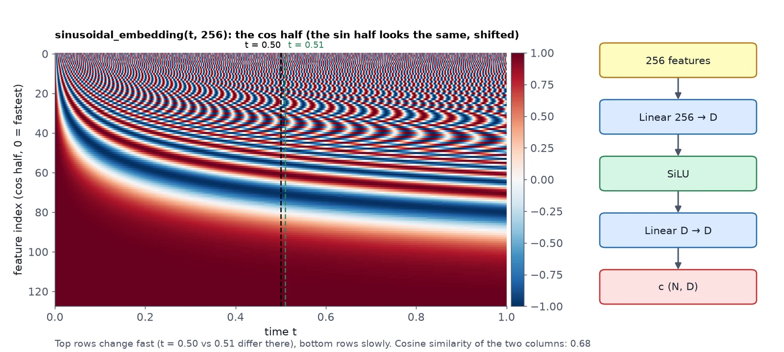
Feeding t as a single number works badly in a big network: one number is easy to drown out, and nearby times like 0.50 and 0.51 look almost identical. Instead we expand t into many sine and cosine waves of different frequencies, the same trick the original Transformer used for positions:
\begin{aligned} \underbrace{\text{emb}(t)}_{256 \text{ numbers}} = \big[&\cos(\omega_0 \cdot 1000t), \dots, \cos(\omega_{127} \cdot 1000t), \\ &\sin(\omega_0 \cdot 1000t), \dots, \sin(\omega_{127} \cdot 1000t)\big] \\ \underbrace{\omega_i = 10000^{-i/128}}_{\text{fast waves} \,\to\, \text{slow waves}} & \end{aligned}Fast waves change a lot between t = 0.50 and t = 0.51, so the model can tell nearby times apart. Slow waves change gently across the whole range, so the model also knows roughly where it is. (We scale t by 1000 so the numbers match the range DiT was designed for.)
In tinydit/model.py, sinusoidal_embedding computes those features:
"""TinyDiT: the simple diffusion transformer (post 9).

x_t (N, 3, 32, 32), t (N,)  ->  predicted velocity (N, 3, 32, 32)
PatchEmbed -> PosEmbed2D -> [DiTBlock(x, c)] x depth -> FinalLayer(x, c) -> unpatchify
c = TimestepEmbedding(t) tells every block how far along the noise line we are.
"""
import math

import torch
from torch import nn

from .attention import MultiHeadAttention
from .config import TinyDiTConfig
from .layers import FeedForward
from .patches import PatchEmbed, PosEmbed2D, unpatchify


def sinusoidal_embedding(t: torch.Tensor, dim: int, max_period: float = 10000.0) -> torch.Tensor:
    """t in [0, 1], shape (N,) -> (N, dim) features [cos(w_i * 1000 t), sin(w_i * 1000 t)]."""
    half = dim // 2
    freqs = torch.exp(-math.log(max_period) * torch.arange(half, device=t.device, dtype=torch.float32) / half)
    args = (1000.0 * t.float())[:, None] * freqs[None, :]      # scale t to the 0..1000 range DiT uses
return torch.cat([torch.cos(args), torch.sin(args)], dim=-1)A small MLP then turns these fixed features into a learned vector c of size D:
class TimestepEmbedding(nn.Module):
    """t (N,) -> c (N, dim): sinusoidal features, then a small MLP."""

    def __init__(self, dim: int, freq_dim: int = 256):
        super().__init__()
        self.freq_dim = freq_dim
        self.mlp = nn.Sequential(nn.Linear(freq_dim, dim), nn.SiLU(), nn.Linear(dim, dim))

    def forward(self, t: torch.Tensor) -> torch.Tensor:
return self.mlp(sinusoidal_embedding(t, self.freq_dim))import torch
import torch.nn.functional as F
from tinydit.model import sinusoidal_embedding, TimestepEmbedding
t = torch.tensor([0.0, 0.01, 0.5, 1.0])
feats = sinusoidal_embedding(t, dim=256)
print("t:", tuple(t.shape), "-> sinusoidal features:", tuple(feats.shape))
print("first 4 features at t=0.5:", [round(v, 3) for v in feats[2, :4].tolist()])
sim = F.cosine_similarity(feats[:, None], feats[None, :], dim=-1)
print("cosine similarity between the four times:")
for i, ti in enumerate(t.tolist()):
print(f" t={ti:<5.2f}", " ".join(f"{s:+.2f}" for s in sim[i].tolist()))
emb = TimestepEmbedding(dim=256)
print("TimestepEmbedding:", tuple(emb(t).shape), "| parameters:", sum(p.numel() for p in emb.parameters()))t: (4,) -> sinusoidal features: (4, 256)
first 4 features at t=0.5: [-0.884, 0.946, 0.849, 0.699]
cosine similarity between the four times:
t=0.00 +1.00 +0.68 +0.27 +0.19
t=0.01 +0.68 +1.00 +0.27 +0.16
t=0.50 +0.27 +0.27 +1.00 +0.27
t=1.00 +0.19 +0.16 +0.27 +1.00
TimestepEmbedding: (4, 256) | parameters: 131584Each time gets its own 256-number fingerprint. Close times (0.00 and 0.01) are fairly similar (0.68), while far-apart times have much lower similarity. That’s the kind of signal a network can easily read.
Timestep embedding: what, why, how
What it is: the layer that turns the time t \in [0, 1] into a vector c the network can use.
Why it works: the right velocity depends on how noisy the input is. Sine and cosine waves at many frequencies give every t a distinct, smooth fingerprint that’s easy for a network to read, and the MLP lets the model learn which aspects of time matter.
How it works: sinusoidal_embedding(t, 256) computes \cos and \sin of 1000t \cdot \omega_i for 128 frequencies. Then Linear(256 → D) → SiLU → Linear(D → D).
What you just built: sinusoidal_embedding and TimestepEmbedding: every t becomes a learned condition vector c of size D.
Step 2/5: Adaptive Layer Norm (adaLN)
In this step: We inject the time vector into every block by letting it set the LayerNorm scale and shift, and build DiTBlock and FinalLayer.
Now every block needs to see c. DiT’s answer is elegant: reuse the LayerNorm that’s already in every block.
A normal LayerNorm (post 5) normalises each token, then applies a learned scale \gamma and shift \beta that are the same for every input. Adaptive LayerNorm computes the scale and shift from the condition instead:
\begin{aligned} \operatorname{adaLN}(x, c) = &\underbrace{\operatorname{LN}(x)}_{\text{normalise, no learned } \gamma, \beta} \odot \big(1 + \underbrace{\text{scale}(c)}_{\text{from a Linear on } c}\big) \\ &+ \underbrace{\text{shift}(c)}_{\text{from a Linear on } c} \end{aligned}The 1 + means that a scale of zero leaves the features unchanged. In code it is one line, modulate:
def modulate(x: torch.Tensor, shift: torch.Tensor, scale: torch.Tensor) -> torch.Tensor:
    """adaLN: x (N, L, D) normalized; shift, scale (N, D) from the condition."""
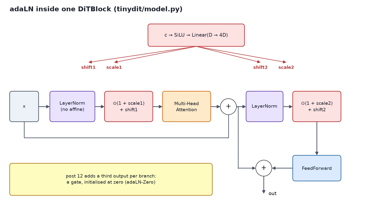
return x * (1 + scale[:, None, :]) + shift[:, None, :]One Linear layer on c produces all the scales and shifts a block needs: one pair for the norm before attention, one pair for the norm before the feed-forward network. That’s DiTBlock:
class DiTBlock(nn.Module):
    """Pre-norm transformer block whose LayerNorms are scaled and shifted by the condition c."""

    def __init__(self, dim: int, num_heads: int, mlp_ratio: float = 4.0, use_sdpa: bool = False):
        super().__init__()
        self.norm1 = nn.LayerNorm(dim, elementwise_affine=False)   # adaLN supplies scale/shift
        self.attn = MultiHeadAttention(dim, num_heads, use_sdpa=use_sdpa)
        self.norm2 = nn.LayerNorm(dim, elementwise_affine=False)
        self.mlp = FeedForward(dim, mlp_ratio)
        self.adaLN = nn.Sequential(nn.SiLU(), nn.Linear(dim, 4 * dim))   # -> shift1, scale1, shift2, scale2

    def forward(self, x: torch.Tensor, c: torch.Tensor) -> torch.Tensor:
        shift1, scale1, shift2, scale2 = self.adaLN(c).chunk(4, dim=-1)
        x = x + self.attn(modulate(self.norm1(x), shift1, scale1))
        x = x + self.mlp(modulate(self.norm2(x), shift2, scale2))
return xDiTBlock is the pre-norm TransformerBlock from post 6 with two changes. Its LayerNorms have elementwise_affine=False, because adaLN supplies the scale and shift. And self.adaLN (a SiLU followed by Linear(D, 4D)) turns c into shift1, scale1, shift2, scale2.
It still uses MultiHeadAttention from post 6 and FeedForward from post 5. Let’s prove the time really changes what a block does:
import torch
from tinydit.model import DiTBlock, TimestepEmbedding, modulate

torch.manual_seed(0)
tokens = torch.randn(2, 64, 256)                    # the SAME tokens for both samples
tokens[1] = tokens[0]
c = TimestepEmbedding(256)(torch.tensor([0.1, 0.9]))   # but two different times

block = DiTBlock(dim=256, num_heads=4)
shift1, scale1, shift2, scale2 = block.adaLN(c).chunk(4, dim=-1)
print("condition c:", tuple(c.shape), "-> shift/scale each:", tuple(shift1.shape))

normed = block.norm1(tokens)
mod = modulate(normed, shift1, scale1)
print("after LayerNorm, samples identical:", torch.allclose(normed[0], normed[1]))
print("after modulate,  samples identical:", torch.allclose(mod[0], mod[1]))
out = block(tokens, c)
print("block output:", tuple(out.shape), "| mean |difference| between t=0.1 and t=0.9:",
      round((out[0] - out[1]).abs().mean().item(), 4))
print("parameters in one DiTBlock:", sum(p.numel() for p in block.parameters()),
"| of which adaLN:", sum(p.numel() for p in block.adaLN.parameters()))condition c: (2, 256) -> shift/scale each: (2, 256)
after LayerNorm, samples identical: True
after modulate, samples identical: False
block output: (2, 64, 256) | mean |difference| between t=0.1 and t=0.9: 0.0159
parameters in one DiTBlock: 1051904 | of which adaLN: 263168The two samples have identical tokens and identical normalised features. Only the time differs, and after modulate they’re different.
Note: One quarter of each block’s parameters (263K of 1.05M) are the adaLN layer. That’s the price of letting the time steer every block.
FinalLayer does the same for the output side: it replaces post 7’s PatchHead LayerNorm with an adaLN, then a Linear(D → 48):
class FinalLayer(nn.Module):
    """adaLN-modulated LayerNorm, then Linear(dim -> p*p*C) per token."""

    def __init__(self, dim: int, patch_size: int, out_channels: int):
        super().__init__()
        self.norm = nn.LayerNorm(dim, elementwise_affine=False)
        self.adaLN = nn.Sequential(nn.SiLU(), nn.Linear(dim, 2 * dim))
        self.proj = nn.Linear(dim, patch_size * patch_size * out_channels)

    def forward(self, x: torch.Tensor, c: torch.Tensor) -> torch.Tensor:
        shift, scale = self.adaLN(c).chunk(2, dim=-1)
return self.proj(modulate(self.norm(x), shift, scale))Adaptive LayerNorm (adaLN): what, why, how
What it is: a way to let the condition (the time now, the class label in post 12) steer every block.
Why it works: scaling and shifting the normalised features changes what the next layer sees, so the same attention and FFN weights can behave differently at t = 0.1 and t = 0.9, with no separate network per time.
How it works: LayerNorm(elementwise_affine=False), then x * (1 + scale) + shift, where shift, scale come from Linear(SiLU(c)). That’s modulate() in model.py.
Why it works: DiT compared this against other ways of injecting the condition (extra tokens, cross-attention) and found adaLN-style conditioning worked best for its class-conditional models.
DiTBlock and FinalLayer: what, why, how
What it is: the repeating unit of TinyDiT, and the output head.
Why it works: they’re the post-6 transformer block and post-7 output head, now time-aware. Attention lets every patch see the whole image, and adaLN tells each block how noisy the image is.
How it works: x = x + attn(modulate(norm1(x))), x = x + mlp(modulate(norm2(x))). FinalLayer: modulate(norm(x)), then Linear(D → 48), then unpatchify.
What you just built: modulate, DiTBlock and FinalLayer: transformer pieces whose behaviour changes with the time t.
Step 3/5: PyTorch DiT: Putting TinyDiT Together
In this step: We assemble the full TinyDiT model and check its shapes and parameter counts.
TinyDiT.forward(x, t) is the architecture diagram written as code: patch embed, add positions, embed the time, run the blocks, then the final layer and unpatchify:
class TinyDiT(nn.Module):
    def __init__(self, cfg: TinyDiTConfig = TinyDiTConfig(), use_sdpa: bool = False):
        super().__init__()
        self.cfg = cfg
        self.embed = PatchEmbed(cfg.img_size, cfg.patch_size, cfg.in_channels, cfg.dim)
        self.pos = PosEmbed2D(cfg.grid_size, cfg.dim)
        self.t_embed = TimestepEmbedding(cfg.dim)
        self.blocks = nn.ModuleList(
            [DiTBlock(cfg.dim, cfg.num_heads, cfg.mlp_ratio, use_sdpa) for _ in range(cfg.depth)])
        self.final = FinalLayer(cfg.dim, cfg.patch_size, cfg.in_channels)

    def forward(self, x: torch.Tensor, t: torch.Tensor) -> torch.Tensor:
        cfg = self.cfg
        h = self.pos(self.embed(x))                 # (N, 64, D)
        c = self.t_embed(t)                         # (N, D)
        for block in self.blocks:
            h = block(h, c)
        out = self.final(h, c)                      # (N, 64, p*p*C)
return unpatchify(out, cfg.patch_size, cfg.in_channels, cfg.img_size, cfg.img_size)Let’s check the shapes and sizes:
import torch
from tinydit import TinyDiTConfig
from tinydit.model import TinyDiT

for name, cfg in [("plan size (Colab GPU)", TinyDiTConfig()),
                  ("CPU size (this post)", TinyDiTConfig(dim=128, depth=4, num_heads=4))]:
    model = TinyDiT(cfg)
    x, t = torch.randn(8, 3, 32, 32), torch.rand(8)
    v = model(x, t)
    print(f"{name}: dim={cfg.dim} depth={cfg.depth} heads={cfg.num_heads} "
          f"| {sum(p.numel() for p in model.parameters()):,} parameters | in {tuple(x.shape)} -> out {tuple(v.shape)}")

print()
for name, p in TinyDiT(TinyDiTConfig(dim=128, depth=4)).named_children():
print(f" {name:8s} {sum(q.numel() for q in p.parameters()):>9,}")plan size (Colab GPU): dim=256 depth=6 heads=4 | 6,603,568 parameters | in (8, 3, 32, 32) -> out (8, 3, 32, 32)
CPU size (this post): dim=128 depth=4 heads=4 | 1,152,176 parameters | in (8, 3, 32, 32) -> out (8, 3, 32, 32)
embed 6,272
pos 2,048
t_embed 49,408
blocks 1,055,232
final 39,216The model takes a noisy image batch and a time per image and returns a tensor of exactly the same shape: the predicted velocity. Nearly all the parameters live in the blocks.
The plan size (dim 256, depth 6, 6.6M parameters) is what we’d train on a GPU. On a CPU we use dim 128 and depth 4, which is about 6× smaller and trains about 4× faster.
| Piece | Built in | Role in TinyDiT |
|---|---|---|
CachedCIFAR10, make_loader | post 4 (+ a cache today) | batches of images in [-1, 1] |
PatchEmbed, PosEmbed2D, unpatchify | post 7 | image ↔ tokens |
MultiHeadAttention, FeedForward | posts 6 and 5 | the inside of each block |
flow_matching_loss, euler_sample | post 8 | what to learn, how to sample |
Trainer | post 5 | the training loop and checkpoints |
TimestepEmbedding, DiTBlock, FinalLayer | today | time-aware blocks |
TinyDiT: what, why, how
What it is: the model that predicts the flow-matching velocity for a noisy image at time t.
Why it works: it’s the DiT recipe (patchify, a stack of adaLN transformer blocks, unpatchify), trained with the straight-line objective that SiT and SD3 use, shrunk to CPU size.
How it works: TinyDiT(cfg)(x_t, t) → velocity of shape (N, 3, 32, 32). Train with Trainer(model, flow_matching_loss), sample with euler_sample(model, noise, steps=20).
What you just built: TinyDiT: (N, 3, 32, 32) noisy images and (N,) times in, (N, 3, 32, 32) velocity out, 1.15M parameters at CPU size.
Step 4/5: Train TinyDiT on CIFAR-10
In this step: We add a fast in-memory CIFAR-10 dataset, train TinyDiT with the post-5 Trainer and the post-8 loss, and watch the same 64 noise images turn into pictures.
One small practical addition first. The post-4 CIFAR loader decodes each image through torchvision transforms, which is fine on a GPU but slow on a CPU.
CachedCIFAR10 loads all 50,000 images once into a single uint8 tensor (about 150 MB), and __getitem__ just scales to [-1, 1] and randomly flips:
class CachedCIFAR10(Dataset):
    """CIFAR-10 held in memory as one uint8 tensor (added in post 9 for fast CPU training).

    Same output as get_cifar10: (image float32 (3, 32, 32) in [-1, 1], label). Train mode adds a
    random horizontal flip. ~150 MB for the 50,000 training images. Use num_workers=0 with it.
    """

    def __init__(self, root: str | Path = "data", train: bool = True,
                 classes: list[int] | None = None, download: bool = True):
        ds = datasets.CIFAR10(root=str(root), train=train, download=download)
        images = torch.from_numpy(ds.data).permute(0, 3, 1, 2).contiguous()   # (N, H, W, C) -> (N, C, H, W)
        labels = torch.tensor(ds.targets, dtype=torch.long)
        if classes is not None:
            keep = torch.isin(labels, torch.tensor(classes))
            images, labels = images[keep], labels[keep]
        self.images, self.labels, self.train = images, labels, train

    def __len__(self) -> int:
        return len(self.labels)

    def __getitem__(self, idx: int) -> tuple[torch.Tensor, torch.Tensor]:
        x = self.images[idx].float() / 127.5 - 1.0                # uint8 [0, 255] -> [-1, 1]
        if self.train and torch.rand(()) < 0.5:
            x = x.flip(-1)                                        # random horizontal flip
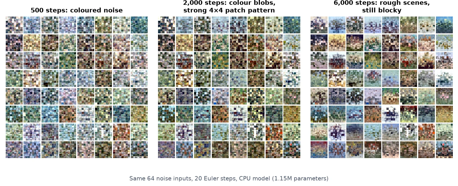
return x, self.labels[idx]Now the training script. It’s the post-5 Trainer with the post-8 loss, nothing new. We stop at 500, 2,000 and 6,000 steps to save a sample grid, always from the same 64 noise images so we can watch the same pictures improve:
import time
import torch
from tinydit import TinyDiTConfig
from tinydit.data import CachedCIFAR10, make_loader
from tinydit.flow import flow_matching_loss, euler_sample
from tinydit.images import save_grid
from tinydit.model import TinyDiT
from tinydit.trainer import Trainer

torch.manual_seed(0)
cfg = TinyDiTConfig(dim=128, depth=4, num_heads=4)          # CPU size; use TinyDiTConfig() on a GPU
model = TinyDiT(cfg)
trainer = Trainer(model, flow_matching_loss, lr=3e-4)
loader = make_loader(CachedCIFAR10("data", train=True), batch_size=128, num_workers=0)
noise = torch.randn(64, 3, 32, 32, generator=torch.Generator().manual_seed(42))   # same noise every time

t0 = time.time()
for checkpoint in [500, 2000, 6000]:
    trainer.fit(loader, max_steps=checkpoint, log_every=500)
    samples = euler_sample(trainer.model, noise, steps=20)
    save_grid(samples, f"samples_step{checkpoint}.png")
    print(f"--- step {checkpoint}: saved samples_step{checkpoint}.png ({time.time() - t0:.0f}s so far)")
trainer.save("checkpoints/tinydit_simple.pt", config=vars(cfg))step 500 | loss 0.4009
--- step 500: saved samples_step500.png (41s so far)
step 1000 | loss 0.3028
step 1500 | loss 0.2900
step 2000 | loss 0.2830
--- step 2000: saved samples_step2000.png (178s so far)
step 2500 | loss 0.2745
step 3000 | loss 0.2654
step 3500 | loss 0.2596
step 4000 | loss 0.2558
step 4500 | loss 0.2511
step 5000 | loss 0.2486
step 5500 | loss 0.2457
step 6000 | loss 0.2433
--- step 6000: saved samples_step6000.png (647s so far)The loss falls quickly to about 0.30, then keeps creeping down. As we saw in post 8, flow-matching loss never reaches zero, so the number to watch is whether it keeps improving and how the samples look.
Note: Train on your own pictures: everything above works with any folder of images, thanks to the ImageFolderDataset from post 4. Swap the dataset line for ImageFolderDataset("my_pictures", img_size=32) and keep the rest. With a small folder (a few hundred photos of one thing, such as cats or one kind of flower) the model has an easier job than all of CIFAR-10, and the samples get recognisable sooner. If you’re short on time, CachedCIFAR10("data", classes=[1]) (cars only) is a similar shortcut.
What you just built: A trained TinyDiT checkpoint (checkpoints/tinydit_simple.pt) and sample grids at 500, 2,000 and 6,000 steps.
Step 5/5: How Good Are These Samples, Honestly?
In this step: We look at the samples honestly and define the two scores, held-out velocity MSE and probe-FD, that every later post uses.
Not very good. After 6,000 steps the grid shows plausible CIFAR-like colour layouts (blue or grey “sky” over brown or green “ground”, a bright blob in the middle of a plain background), but you can’t name the objects, and you can clearly see the 4×4 patch grid.
That’s expected for this budget: 6,000 steps × 128 images is about 15 passes over CIFAR-10 with a 1.15M-parameter model. The DiT paper trained for 400,000 steps or more, with models up to 675M parameters. Our job here is a working, honest baseline, not a pretty one.
To compare models in later posts we need numbers, not just eyeballing. We use two:
- Held-out velocity MSE. The flow-matching loss on 2,000 CIFAR-10 test images, with the noise and the times fixed by a seed, so every model is scored on exactly the same questions. Lower is better.
- probe-FD. The standard image-quality score is FID: run real and generated images through a big pretrained network (Inception) and compare the statistics of its features. We don’t want a big pretrained dependency, so we trained a small CIFAR-10 classifier once (87% test accuracy, in
tinydit/metrics.py) and compute the same Fréchet distance on its features. Lower is better.
Watch out: probe-FD is not FID, and the numbers can’t be compared with FID in papers. It does rank our own models consistently.
First, the held-out velocity MSE of the trained model against an untrained one:
import torch
from tinydit import TinyDiTConfig
from tinydit.data import CachedCIFAR10
from tinydit.flow import euler_sample
from tinydit.metrics import velocity_mse, load_probe, probe_features, probe_scores
from tinydit.model import TinyDiT

ckpt = torch.load("checkpoints/tinydit_simple.pt", weights_only=True)
model = TinyDiT(TinyDiTConfig(**ckpt["config"]))
model.load_state_dict(ckpt["model"])

test = CachedCIFAR10("data", train=False)
test_x = test.images[:2000].float() / 127.5 - 1
untrained = TinyDiT(TinyDiTConfig(**ckpt["config"]))
print(f"held-out velocity MSE: untrained {velocity_mse(untrained, test_x):.4f} | trained {velocity_mse(model, test_x):.4f}")Then probe-FD for real images, pure noise, and TinyDiT samples at 5, 20 and 50 steps, plus what the probe thinks the samples are:
probe = load_probe("probe.pt")                                   # our small CIFAR classifier, used only as a ruler
real_feats = torch.load("probe_real_feats.pt", weights_only=True)  # probe features of the 10,000 test images
train_x = CachedCIFAR10("data", train=True).images[:1000].float() / 127.5 - 1
noise = torch.randn(1000, 3, 32, 32, generator=torch.Generator().manual_seed(0))
print("probe-FD (lower = closer to real CIFAR-10 test images, 1,000 images each):")
print(f"  real training images : {probe_scores(probe, train_x, real_feats)['probe_fd']:.1f}   <- best we could hope for")
print(f"  pure noise           : {probe_scores(probe, noise.clamp(-1, 1), real_feats)['probe_fd']:.1f}")
for steps in [5, 20, 50]:
    samples = torch.cat([euler_sample(model, noise[i:i + 250], steps=steps) for i in range(0, 1000, 250)])
    print(f"  TinyDiT, {steps:2d} steps   : {probe_scores(probe, samples, real_feats)['probe_fd']:.1f}")

_, logits = probe_features(probe, samples)
counts = torch.bincount(logits.argmax(1), minlength=10)
names = ["plane", "car", "bird", "cat", "deer", "dog", "frog", "horse", "ship", "truck"]
print("what the probe thinks the 50-step samples are:", ", ".join(f"{n} {c}" for n, c in zip(names, counts.tolist())))held-out velocity MSE: untrained 1.5556 | trained 0.2446
probe-FD (lower = closer to real CIFAR-10 test images, 1,000 images each):
real training images : 0.6 <- best we could hope for
pure noise : 167.5
TinyDiT, 5 steps : 73.1
TinyDiT, 20 steps : 67.3
TinyDiT, 50 steps : 66.4
what the probe thinks the 50-step samples are: plane 51, car 0, bird 21, cat 35, deer 231, dog 0, frog 55, horse 48, ship 238, truck 321The trained model’s velocity MSE (0.245) is far below the untrained one (1.56). On probe-FD our samples (66 at 50 steps) sit much closer to real images than pure noise does (168), but nowhere near real training images (0.6). There’s a lot of room left, which is what posts 11 to 14 are for.
Two more honest observations:
- More sampling steps help a little (73 → 67 → 66 for 5, 20 and 50 steps). The path is fairly smooth, so 20 steps already gets most of the benefit. We’ll use 20 from now on.
- The probe labels most samples as trucks, ships and deer. That isn’t because the model draws trucks. It’s because blurry blobs on plain backgrounds look most like those classes to a classifier. The model doesn’t know about classes at all yet; post 12 teaches it.
What you just built: The “before” numbers for every Expert post: velocity MSE 0.245 (untrained: 1.56) and probe-FD 67 at 20 steps (noise: 168, real images: 0.6).
Recap
- A PyTorch DiT needs to know the time: a timestep embedding (sinusoidal features + MLP) turns t into a vector c.
- adaLN injects c into every block: normalise, then
x * (1 + scale(c)) + shift(c). - TinyDiT = PatchEmbed → positions → DiTBlocks → FinalLayer → unpatchify. 1.15M parameters at CPU size.
- 6,000 CPU steps (11 minutes): velocity MSE 0.245 (untrained: 1.56) and probe-FD 67 at 20 steps (noise: 168, real images: 0.6). The samples are blurry, blocky colour layouts, honestly not objects yet.
- This checkpoint and these numbers are the “before” for every Expert post.
Next up: In torch.compile, Mixed Precision, and SDPA: Speed Up TinyDiT we make training faster with three PyTorch 2 tools, SDPA, mixed precision and torch.compile, and measure what each one really buys on a CPU.
Series: PyTorch Tutorial 2026 (14 posts)
- Post 1: PyTorch Tutorial 2026: From Tensors to Tiny Diffusion
- Post 2: PyTorch Tensors Explained: Shapes, Broadcasting, and Images as Arrays
- Post 3: PyTorch Autograd: How backward() Builds Gradients
- Post 4: PyTorch DataLoader Explained: Datasets, Batches, and Image Folders
- Post 5: PyTorch nn.Module and the Training Loop: Layers, Loss, and Checkpoints
- Post 6: Attention and the Transformer Block in PyTorch
- Post 7: Patch Embeddings in PyTorch: How a Transformer Reads an Image
- Post 8: Flow Matching in PyTorch: Train a Model to Follow a Straight Line
- Post 9: Build a Tiny Diffusion Transformer in PyTorch (DiT from Scratch) (you are here)
- Post 10: torch.compile, Mixed Precision, and SDPA: Speed Up TinyDiT
- Post 11: RMSNorm, QK-Norm, SwiGLU, and 2D RoPE in a Tiny DiT
- Post 12: adaLN-Zero and Classifier-Free Guidance in PyTorch
- Post 13: MMDiT Joint Attention in PyTorch: Two Streams, One Generator
- Post 14: Train and Sample Like 2026: Logit-Normal Steps, EMA, and Few-Step Flow
← Previous: Post 8: Flow Matching in PyTorch: Train a Model to Follow a Straight Line
Next → Post 10: torch.compile, Mixed Precision, and SDPA: Speed Up TinyDiT