PyTorch Tutorial 2026: From Tensors to Tiny Diffusion

In this post:

• Introduction
• Step 1/6: What You Will Build in This PyTorch Tutorial
• Step 2/6: What Is PyTorch in 2026?
• Step 3/6: Colab or Local? Install PyTorch
• Step 4/6: Check Your Install and Your GPU
• Step 5/6: Your First Tensor
• Step 6/6: How to Follow the Series
• Recap

Introduction

Welcome to PyTorch Tutorial 2026: From Tensors to Tiny Diffusion. This pytorch tutorial series takes you from your very first tensor all the way to a small image generator that you write yourself, line by line.

No copy-pasting a giant repo you don’t understand. We build one project, called TinyDiT, and every post adds one real piece of it.

TinyDiT is a tiny version of the kind of model behind Stable Diffusion 3 and FLUX: a Diffusion Transformer (DiT) trained with flow matching. It is small enough to train on a free Google Colab GPU, and the first version even runs (slowly) on a laptop CPU.

Once the simple version works, the Expert part of the series upgrades it with the layers that current state-of-the-art models use, one at a time, and measures what each one actually does.

In this first post we install PyTorch, check which device you have, and make your first tensor. This page is also the hub of the series, so the full table of contents is in the last step.

Step 1/6: What You Will Build in This PyTorch Tutorial

In this step: We describe the finished TinyDiT project in one sentence and map each idea in it to the post that teaches it.

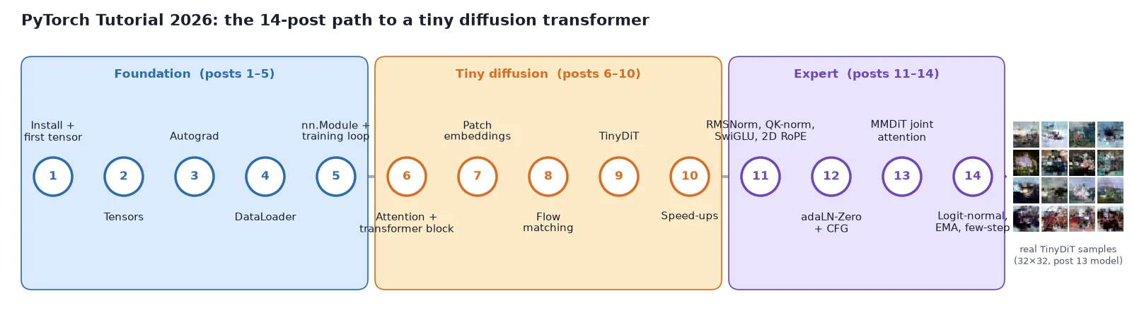
Here is the finished project in one sentence: a transformer that looks at a noisy picture, cut into small patches, and predicts which direction to move each pixel to make it look more like a real image. Repeat that small step 20 times starting from pure noise, and a picture appears.

That one sentence hides every important idea in modern image generation:

• Tensors hold the images, the noise, and the model’s weights (posts 1–2).
• Autograd computes how to change millions of weights to reduce the error (post 3).
• Datasets and DataLoaders feed the model batches of images (post 4).
• nn.Module and a training loop turn layers into a model and a model into something that learns (post 5).
• Attention and the transformer block let every part of the picture look at every other part (post 6).
• Patch embeddings turn a picture into a sequence of tokens a transformer can read (post 7).
• Flow matching gives the model a simple target: the straight-line direction from image to noise (post 8).
• TinyDiT wires everything together and generates its first images (post 9), then gets faster with torch.compile, mixed precision and fused attention (post 10).
• Expert upgrades: RMSNorm, QK-norm, SwiGLU, 2D RoPE, adaLN-Zero, classifier-free guidance, MMDiT joint attention, logit-normal timesteps, EMA, and few-step sampling (posts 11–14).

We train on CIFAR-10, a classic dataset of 60,000 tiny 32×32 color pictures in 10 classes (planes, cars, birds, cats…). Small pictures keep training cheap, and you will be able to point the same code at your own image folder later.

Step 2/6: What Is PyTorch in 2026?

In this step: We see what PyTorch actually does, the four moves of training a network, and which PyTorch version this series uses.

PyTorch is a Python library for doing math on big arrays of numbers, on a CPU or a GPU, and for automatically computing gradients of that math. Those two features are all you need to train a neural network:

1. Store data and model weights as arrays (PyTorch calls them tensors).
2. Compute a prediction and measure how wrong it is (the loss).
3. Ask PyTorch for the gradient of the loss with respect to every weight.
4. Nudge every weight a little in the direction that reduces the loss. Repeat.

On top of that core, PyTorch gives you ready-made layers (torch.nn), optimizers (torch.optim) and data loading (torch.utils.data). The 2.x releases add speed tools like torch.compile, mixed precision (torch.amp) and fused attention (F.scaled_dot_product_attention). We will use all of these, each when it is needed.

This series targets PyTorch 2.15, the current stable release (announced on the official PyTorch blog on 28 October 2026). Every code block in these posts was run with PyTorch 2.15.0 on Python 3.13, so the outputs you see are real.

Step 3/6: Colab or Local? Install PyTorch

In this step: We pick where your code will run, a free Colab GPU or your own machine, and install PyTorch there.

You have two easy options. You do not need to buy a GPU for this series.

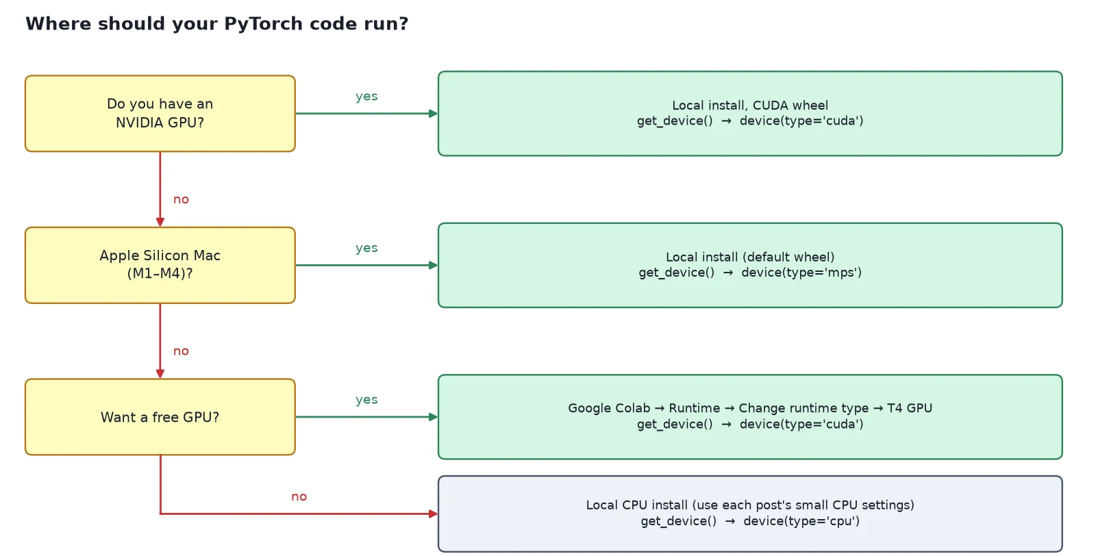
Option 1: Google Colab (recommended for beginners)

Go to colab.research.google.com, create a new notebook, then choose Runtime → Change runtime type → T4 GPU. PyTorch is already installed.

In the first cell, print the version and check that the GPU is visible:

import torch
print(torch.__version__)
print(torch.cuda.is_available())

import torch
print(torch.__version__)
print(torch.cuda.is_available())

If the version printed is older than 2.15, run !pip install -U torch torchvision in a cell and restart the runtime.

Option 2: Install PyTorch locally

You need Python 3.11 or newer (PyTorch 2.15 supports 3.11 to 3.15). Make a fresh virtual environment so PyTorch does not fight with other projects:

# 1) Create and activate a virtual environment
python3 -m venv .venv
source .venv/bin/activate          # Windows: .venv\Scripts\activate

# 2a) Linux with an NVIDIA GPU, or macOS (Apple Silicon uses "mps" automatically):
pip install torch torchvision

# 2b) CPU-only machine (smaller download):
pip install torch torchvision --index-url https://download.pytorch.org/whl/cpu

# 3) Check it worked
python -c "import torch; print(torch.__version__)"

# 1) Create and activate a virtual environment
python3 -m venv .venv
source .venv/bin/activate          # Windows: .venv\Scripts\activate

# 2a) Linux with an NVIDIA GPU, or macOS (Apple Silicon uses "mps" automatically):
pip install torch torchvision

# 2b) CPU-only machine (smaller download):
pip install torch torchvision --index-url https://download.pytorch.org/whl/cpu

# 3) Check it worked
python -c "import torch; print(torch.__version__)"

Step 4/6: Check Your Install and Your GPU

In this step: We write the first file of the TinyDiT repo, which prints your PyTorch version and picks the best device.

This is the very first file of the TinyDiT repo, hello_torch.py. It starts with a function that picks the best device:

"""hello_torch.py - commit one of the TinyDiT repo.

Prints the PyTorch version, the best available device, and a 3x3 tensor.
Run:  python hello_torch.py
"""
import torch


def pick_device() -> torch.device:
    """Prefer an NVIDIA/AMD GPU (cuda), then Apple Silicon (mps), then CPU."""
    if torch.cuda.is_available():
        return torch.device("cuda")
    if torch.backends.mps.is_available():
        return torch.device("mps")
    return torch.device("cpu")

"""hello_torch.py - commit one of the TinyDiT repo.

Prints the PyTorch version, the best available device, and a 3x3 tensor.
Run:  python hello_torch.py
"""
import torch


def pick_device() -> torch.device:
    """Prefer an NVIDIA/AMD GPU (cuda), then Apple Silicon (mps), then CPU."""
    if torch.cuda.is_available():
        return torch.device("cuda")
    if torch.backends.mps.is_available():
        return torch.device("mps")
    return torch.device("cpu")

The main block prints the version and the device, then makes a small random tensor on it:

if __name__ == "__main__":
    device = pick_device()
    print("PyTorch version:", torch.__version__)
    print("Device:", device)
    if device.type == "cuda":
        print("GPU:", torch.cuda.get_device_name(0))

    x = torch.rand(3, 3, device=device)
    print(x)
    print("shape:", tuple(x.shape), "| dtype:", x.dtype, "| device:", x.device)

if __name__ == "__main__":
    device = pick_device()
    print("PyTorch version:", torch.__version__)
    print("Device:", device)
    if device.type == "cuda":
        print("GPU:", torch.cuda.get_device_name(0))

    x = torch.rand(3, 3, device=device)
    print(x)
    print("shape:", tuple(x.shape), "| dtype:", x.dtype, "| device:", x.device)

Run it with python hello_torch.py. On my test machine (CPU only) the output is:

PyTorch version: 2.15.0+cpu
Device: cpu
tensor([[0.8110, 0.5316, 0.1587],
        [0.4307, 0.2078, 0.4103],
        [0.9693, 0.8319, 0.7084]])
shape: (3, 3) | dtype: torch.float32 | device: cpu

On a Colab T4 you will see Device: cuda and GPU: Tesla T4. On an Apple Silicon Mac you will see Device: mps. All three are fine.

The device logic picks cuda first (NVIDIA GPUs, and AMD GPUs through ROCm builds, both show up as cuda), then mps (Apple’s Metal backend), then falls back to cpu. The repo keeps the same logic in tinydit/device.py, so every later script can just call get_device():

"""Device helper used by every script in the series (post 1)."""
import torch


def get_device(prefer: str | None = None) -> torch.device:
    """Return the best device: cuda > mps > cpu.

    Pass prefer="cpu" (or "cuda", "mps") to force one.
    """
    if prefer is not None:
        return torch.device(prefer)
    if torch.cuda.is_available():
        return torch.device("cuda")
    if torch.backends.mps.is_available():
        return torch.device("mps")
    return torch.device("cpu")

"""Device helper used by every script in the series (post 1)."""
import torch


def get_device(prefer: str | None = None) -> torch.device:
    """Return the best device: cuda > mps > cpu.

    Pass prefer="cpu" (or "cuda", "mps") to force one.
    """
    if prefer is not None:
        return torch.device(prefer)
    if torch.cuda.is_available():
        return torch.device("cuda")
    if torch.backends.mps.is_available():
        return torch.device("mps")
    return torch.device("cpu")

Step 5/6: Your First Tensor

In this step: We meet the tensor, the one object everything in PyTorch is made of, and do our first math and device moves with it.

Whenever this series introduces a new layer, block or training piece, it gets three labeled answers: What it is, Why it works, and How it works. This post adds no neural-network layer yet, so we start with the tensor.

What it is

A tensor is the array PyTorch computes on. A single number, a list of numbers, a table, a stack of color images, the weights of a layer, and the gradients of those weights are all tensors.

In TinyDiT, the input picture, the noise, the predicted velocity and every weight will be tensors.

Why it works

A plain Python list can store numbers, but it cannot run on a GPU, it does not know its own number type, and it cannot track gradients. A tensor carries three extra facts with the numbers:

• shape: how many numbers along each axis, for example (2, 3) for 2 rows and 3 columns;
• dtype: the number type, usually float32 for model math and int64 for labels;
• device: where the numbers live (cpu, cuda, or mps).

Because data, weights and gradients all share this one format, PyTorch can push the whole computation to a GPU and differentiate through it automatically.

How it works

You make a tensor from a Python list with torch.tensor, or ask for one filled with zeros, ones or random numbers:

import torch

torch.manual_seed(0)                 # same "random" numbers every run

a = torch.tensor([[1.0, 2.0, 3.0],
                  [4.0, 5.0, 6.0]])  # from a Python list
b = torch.rand(2, 3)                 # uniform random numbers in [0, 1)
c = torch.zeros(2, 3)
d = torch.ones(2, 3, dtype=torch.int64)

print(a)
print("shape:", a.shape, "| dtype:", a.dtype, "| device:", a.device)
print(b)
print(c)
print(d, d.dtype)

import torch

torch.manual_seed(0)                 # same "random" numbers every run

a = torch.tensor([[1.0, 2.0, 3.0],
                  [4.0, 5.0, 6.0]])  # from a Python list
b = torch.rand(2, 3)                 # uniform random numbers in [0, 1)
c = torch.zeros(2, 3)
d = torch.ones(2, 3, dtype=torch.int64)

print(a)
print("shape:", a.shape, "| dtype:", a.dtype, "| device:", a.device)
print(b)
print(c)
print(d, d.dtype)

tensor([[1., 2., 3.],
        [4., 5., 6.]])
shape: torch.Size([2, 3]) | dtype: torch.float32 | device: cpu
tensor([[0.4963, 0.7682, 0.0885],
        [0.1320, 0.3074, 0.6341]])
tensor([[0., 0., 0.],
        [0., 0., 0.]])
tensor([[1, 1, 1],
        [1, 1, 1]]) torch.int64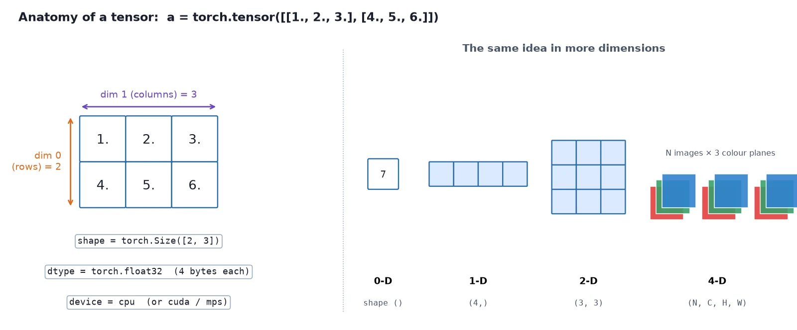

Tensors support the math you would expect. Operators like + and * work element by element, and @ is matrix multiplication:

import torch

a = torch.tensor([[1.0, 2.0, 3.0],
                  [4.0, 5.0, 6.0]])

print(a + 10)          # add to every element
print(a * a)           # element-wise multiply
print(a.sum(), a.mean())
print(a @ a.T)         # matrix multiply: (2, 3) @ (3, 2) -> (2, 2)
print(a[1, 2])         # row 1, column 2 -> 6.0
print(a[1, 2].item())  # a plain Python float

import torch

a = torch.tensor([[1.0, 2.0, 3.0],
                  [4.0, 5.0, 6.0]])

print(a + 10)          # add to every element
print(a * a)           # element-wise multiply
print(a.sum(), a.mean())
print(a @ a.T)         # matrix multiply: (2, 3) @ (3, 2) -> (2, 2)
print(a[1, 2])         # row 1, column 2 -> 6.0
print(a[1, 2].item())  # a plain Python float

tensor([[11., 12., 13.],
        [14., 15., 16.]])
tensor([[ 1.,  4.,  9.],
        [16., 25., 36.]])
tensor(21.) tensor(3.5000)
tensor([[14., 32.],
        [32., 77.]])
tensor(6.)
6.0

Matrix multiplication is the workhorse of deep learning. The shapes must line up: for A @ B, the last axis of A must match the first axis of B.

(2 \times \underbrace{3}_{\text{must match}}) \;@\; (\underbrace{3}_{\text{must match}} \times 2) \;\rightarrow\; (2 \times 2)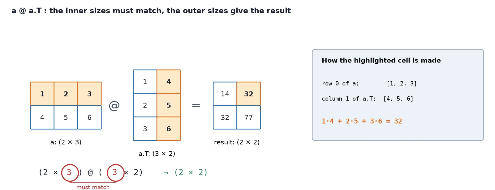

Finally, moving a tensor to the GPU is one call:

import torch
from tinydit import get_device

device = get_device()               # cuda > mps > cpu
x = torch.rand(3, 3).to(device)     # move a tensor to the device
y = torch.rand(3, 3, device=device) # or create it there directly
z = x @ y                           # both on the same device, so this works
print(z.device)
print(z.cpu().shape)                # .cpu() brings it back, e.g. to save or plot

import torch
from tinydit import get_device

device = get_device()               # cuda > mps > cpu
x = torch.rand(3, 3).to(device)     # move a tensor to the device
y = torch.rand(3, 3, device=device) # or create it there directly
z = x @ y                           # both on the same device, so this works
print(z.device)
print(z.cpu().shape)                # .cpu() brings it back, e.g. to save or plot

cpu
torch.Size([3, 3])

Step 6/6: How to Follow the Series

In this step: We cover how the series is meant to be read, what the repo looks like, and the full table of contents.

• One repo, one project. Every post adds files to the same tinydit repo. Nothing is a throwaway example; later posts import what earlier posts built.
• Read in order the first time. Each post assumes the previous ones. After that, the table below makes a good reference.
• Run the code. Each snippet is short and was tested exactly as shown. Typing it out (instead of pasting) is the fastest way to learn the APIs.
• Every new layer gets a What it is / Why it works / How it works. If something feels like magic, that part is where to look.

By the end of post 7, the repo looks like this. Posts 8–14 add the flow-matching loss, the TinyDiT model, and the expert upgrades.

tinydit-repo/
├── hello_torch.py        # post 1: version + device check
├── examples/             # posts 3, 5, 7: fit_line.py, patch_denoiser.py, image_denoiser.py
└── tinydit/
    ├── __init__.py
    ├── device.py         # post 1: get_device()
    ├── config.py         # post 7: TinyDiTConfig (sizes used all series)
    ├── images.py         # post 2: image <-> tensor utilities
    ├── data.py           # post 4: CIFAR-10 + image-folder loaders
    ├── layers.py         # post 5: FeedForward, ResidualFFN
    ├── trainer.py        # post 5: Trainer with checkpoints
    ├── attention.py      # post 6: MultiHeadAttention
    ├── blocks.py         # post 6: TransformerBlock
    └── patches.py        # post 7: patchify, PatchEmbed, PosEmbed2D, PatchHead

The complete series: table of contents

Recap

• PyTorch is tensors plus automatic gradients, with layers, optimizers, data tools and compilers on top.
• Use Colab (free T4 GPU) or a local install with Python 3.11+. The official selector gives the exact install command.
• get_device() picks cuda, then mps, then cpu. Tensors that meet in one operation must share a device.
• A tensor is numbers plus a shape, a dtype and a device.
• Over 14 posts we build TinyDiT, a small diffusion transformer trained with flow matching, then upgrade it with the layers current models use.

Next up: In PyTorch Tensors Explained: Shapes, Broadcasting, and Images as Arrays: shapes, broadcasting, and how a photo becomes an (N, C, H, W) tensor. That file, tinydit/images.py, is the first module the whole project imports.

Next → Post 2: PyTorch Tensors Explained: Shapes, Broadcasting, and Images as Arrays